Gating Cells in cytoverse

Background

The purpose of flow cytometry is to make inferences regarding some cell type(s) of interest. Often this involves establishing/drawing a gating hierarchy to sequentially filter down to the cell type(s) of interest. This process is very often done manually, and can be very labour intensive. Importantly, manual approach implies large variation when one person does it vs. the next, or even if the same person does it multiple times. The cytoverse offers a suite of tools to tackle this problem in a reproducible and programmatic manner.

GatingSet and GatingHeirarchy

In the previous sections, we have seen (and worked with) cytoframe, and cytoset. These objects hold the underlying data, allowing us to visualize it, manipulate it, etc.

In this section we work with GatingSet and GatingHierarchy. These objects, like the name suggests, store information regarding various gates and filters that we will generate. Importantly, we can save the GatingSet which will completely package the analysis as well as the .fcs files in an opensource format that can be shared, allowing reproducibility.

In part 1 of this section, we will go over variety of native methods that exist in the cytoverse which analysts can utilize to gate their cells of interest.

In part 2 of this sections, we will go over methods to extract gated data for cells/populations of interest.

In part 3 (optional), we will demonstrate how analysts can automate this process by utilizing a gatingTemplate (a csv file that can be used to define and build the hierarchy).

Creating a `GatingSet`

Required libraries

library(flowWorkspace)
library(ggcyto)
# set ggcyto theme  
theme_set(theme_classic())
library(CytoverseBioc2023)

## Warning: replacing previous import 'flowViz::contour' by 'graphics::contour'
## when loading 'flowStats'

cache_workshop_data()

To create a GatingSet, first load in a cytoset. Here, we are making use of the cytoset that we have created previously.

# load cytoset
cs <- make_cytoset(only_TNK = TRUE)

# creating a GatingSet
gs <- flowWorkspace::GatingSet(cs)
gs

## A GatingSet with 4 samples

We have now created a GatingSet called gs.

Exercise

How would you check the metadata associated with the GatingSet?
How would you subset gs to only include samples where Treatment = Control?

The GatingSet needs to be compensated and transformed before we start attaching gates.

Note: The approach to compensate and transform a GatingSet is similar to that of cytoframe and cytoset; As such, we ask you to run the code below, up to line 125.

We can directly compensate the GatingSet object.

# compensate a GatingSet
spill <- keyword(gs[[1]],"$SPILLOVER") # extract spillover matrix stored within the file

gs <- compensate(gs,spill) # GatingSet will be compensated and stores the spill matrix as well

recompute(gs) # update the gs

# retrieve compensation information
gs_spill <- gs_get_compensations(gs[[1]])

# output is a rich spillover information
slot(gs_spill[[1]],"spillover")[1:4, 1:4]

##             B515-A     B610-A     B660-A      B710-A
## B515-A 1.000000000 0.07573059 0.04266579 0.003687143
## B610-A 0.009777704 1.00000000 0.78589800 0.074328487
## B660-A 0.005482375 0.03108691 1.00000000 0.112570733
## B710-A 0.024698965 0.12699130 0.90643808 1.000000000

As well we can transform the GatingSet.

For convenience, we are using a previously defined transformerList object. The transformerList object was extracted from the workspace file created by the authors of this study and can be found here.

# transformation of GatingSet
t.rds <- dplyr::filter(
  get_workshop_data("/fj_wsp"), # a previously defined transformation
  grepl(
    pattern = "transform", 
    x = rname
  )
)$rpath
my_trans <- readRDS(file = t.rds)

# make into transformerList object
my_trans_list <- flowWorkspace::transformerList(
  from = names(my_trans),
  trans = my_trans
)

gs <- flowWorkspace::transform(gs, my_trans_list) # transforms underlying data

Exercise

How would you be able to tell if a GatingSet has been compensated?
How would be able to tell if a GatingSet has been transformed? Hint: Try help.search("get_transformation").
Why might it be beneficial to compensate and transform a GatingSet rather than a cytoframe or a cytoset?

A note about `GatingHierarchy`

You may have noticed above that some function calls have gs_ and others have gh_.

gs_ indicates that GatingSet while gh_ indicates a GatingHierarchy.

The GatingHierarchy is a data structure that stores the sample-wise gating information present in a GatingSet. In essence a GatingSet is a collection of GatingHierarchy.

You can access the GatingHierarchy using the [[ subset operation.

Exercise

Try running gh_get_compensations(gs). Why do you get an error message? How would you fix this?
What other methods have gs_ and gh_?
What is the difference between gs[1] and gs[[1]]?
Why are there multiple data structures to represent and hold flow cytometry data in the cytoverse?

Adding gates and building a hierarchy

On this GatingSet, we will add various gates that identifies cells of interest. Each sample within a GatingSet is associated with a GatingHierarchy that stores information regarding various gates that we would have created and applied to the samples.

Below, we demonstrate various types of gates that could be estimated automatically or be defined programmatically which can be applied to the samples within a GatingSet to build a hierarchy.

Note: This process is informed by visualization of the data. As such, we will make ample use of the ggcyto library.

Automatic estimation of gates

The gs_add_gating_method call from openCyto library can be leveraged for automatic estimation of gates, as well as clean scripting! Available gating methods can be listed by calling gt_list_methods(). Please see additional examples here: cytoverse.

List of available methods.

## Gating Functions:
## ===  quantileGate 
## ===  gate_quantile 
## ===  rangeGate 
## ===  flowClust.2d 
## ===  gate_flowclust_2d 
## ===  mindensity 
## ===  gate_mindensity 
## ===  mindensity2 
## ===  gate_mindensity2 
## ===  cytokine 
## ===  flowClust.1d 
## ===  gate_flowclust_1d 
## ===  boundary 
## ===  singletGate 
## ===  quadGate.tmix 
## ===  gate_quad_tmix 
## ===  quadGate.seq 
## ===  gate_quad_sequential 
## Preprocessing Functions:
## ===  prior_flowClust 
## ===  prior_flowClust 
## ===  warpSet 
## ===  standardize_flowset

Singlets gate

A singlets gate is mostly used for data clean up, by removing out doublets.

# visualization
singlet_vis <- autoplot(
  gs_pop_get_data(gs,"root"), # gs_pop_get_data(gs, node) extracts the underlying data
  x = "FSC-A",
  y = "FSC-H",
  bins = 256
  ) +
  facet_wrap(~sampleNames(gs)
  ) # leverage the metadata that is saved within the GatingSet to facet plots 
singlet_vis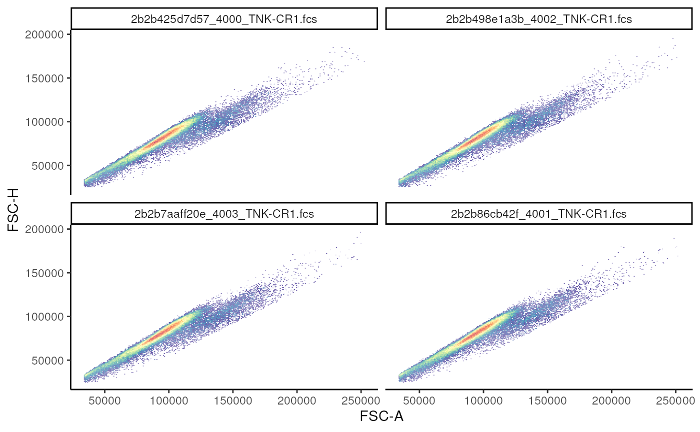

Now, we estimate and add!

# estimate and add
gs_add_gating_method(
  gs = gs, # gatingset
  alias = "singlets", # name given to the population
  pop = "+", # indicate whether events inside or outside the gate should be filtered
  parent = "root", # where to attach this node
  dims = "FSC-A,FSC-H", # dimensions used to estimate the gate
  gating_method = "singletGate", # one of the available gating methods
  gating_args = "wider_gate = FALSE", # arguments passed to singletGate
)
# visualize
singlet_vis + 
  geom_gate(
    gs_pop_get_gate(
      gs,
      "singlets"
    )
  )+
  facet_wrap(~name)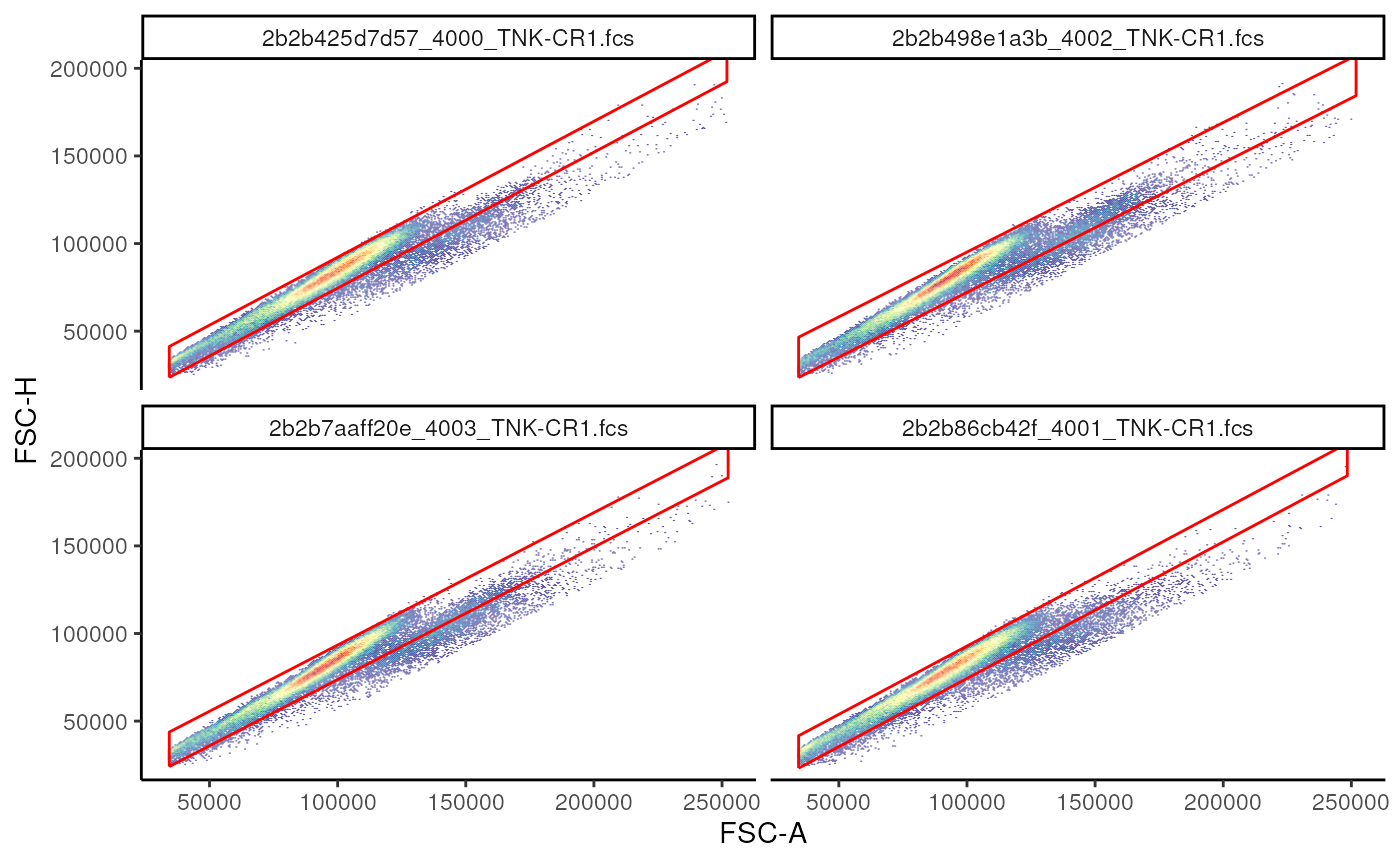

Estimating cutpoint and ranges using `gate_quantile` and `gate_mindensity2`

gate_quantile and gate_mindensity2 can be used to estimate a cut point in the data, allowing the gating of data to the left(-) or the right(+) of the cut point.

# calculate a live gate 
## Example of a quantile gate

## visualize
live_viz <- ggcyto(
  gs,
  subset = "singlets",
  aes(x = "Live", y = "FSC-A")
) +
geom_hex(bins = 128)+
facet_wrap(~name)
# live_viz

# add gate using gate_quantile
gs_add_gating_method(
  gs,
  alias = "live",
  pop = "-",
  parent = "singlets",
  dims = "U450-A",
  gating_method = "gate_quantile",
  gating_args = list(
    probs = 0.95
  )
)

# add gate using gate_mindensity2
gs_add_gating_method(
  gs,
  alias = "live_mindensity",
  pop = "-",
  parent = "singlets",
  dims = "U450-A",
  gating_method = "gate_mindensity2",
  gating_args = list(
    max = 100, 
    gate_range = c(50, 75)
  )
)

# visualize the 2 extimated gates
live_viz+
  geom_gate(gs_pop_get_gate(gs, "live"), colour = "red")+
  geom_gate(gs_pop_get_gate(gs, "live_mindensity"), colour = "blue")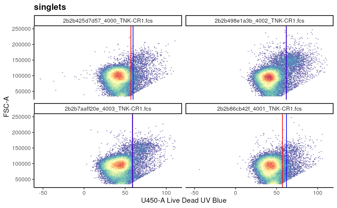

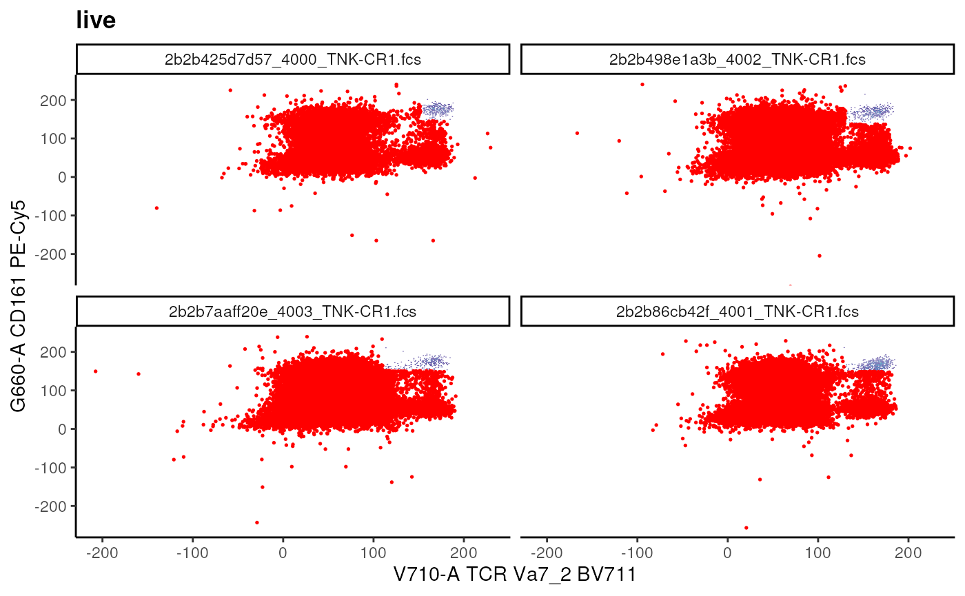
We can also use the cutpoints to estimate a rectangular gate!

# conventional T cells
t_cell_vis <- ggcyto(
  gs, subset = "live",
  aes(x  = "TCR Va7_2", y = "CD161")
) + geom_hex(bins = 256)+
  facet_wrap(~name)

# visualize 
# t_cell_vis

# estimate and add
gs_add_gating_method(
  gs,
  alias = "MAIT Cells",
  pop = "++",
  parent = "live",
  dims = "G660-A,V710-A",
  gating_method = "gate_quantile",
  gating_args = list(
    probs = 0.95, 
    min = 50, 
    max = 200
  )
)

## ...

## done

# visualize
t_cell_vis+
  geom_gate(gs_pop_get_gate(gs,"MAIT Cells"))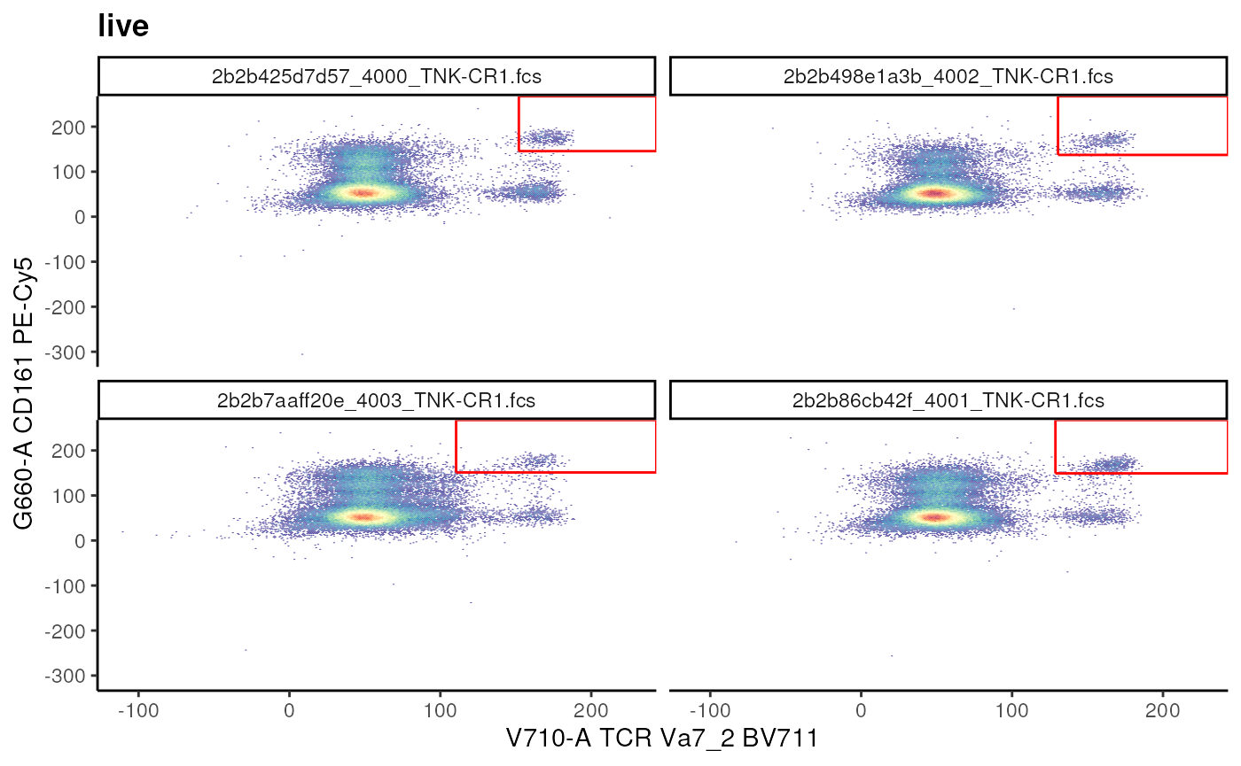

Estimating an Ellipsoid gate

gate_flowclust_2d can be used to identify and generate an Ellipsoid gate in a semi-supervised manner.

cd3_ellipse <- ggcyto(gs,
       subset = "live",
       aes(x = "CD4", y = "CD3"))+
  geom_hex(bins = 256)

# estimate and add
gs_add_gating_method(
  gs,
  alias = "CD3+",
  pop = "+",
  parent = "live",
  dims = "U785-A,V510-A",
  gating_method = "gate_flowclust_2d",
  gating_args = list(
    K = 3,
    target = c(100,150),
    quantile = 0.9,
    plot = FALSE
  )
)

# visualize
cd3_ellipse+
  geom_gate(gs_pop_get_gate(gs,"CD3+"))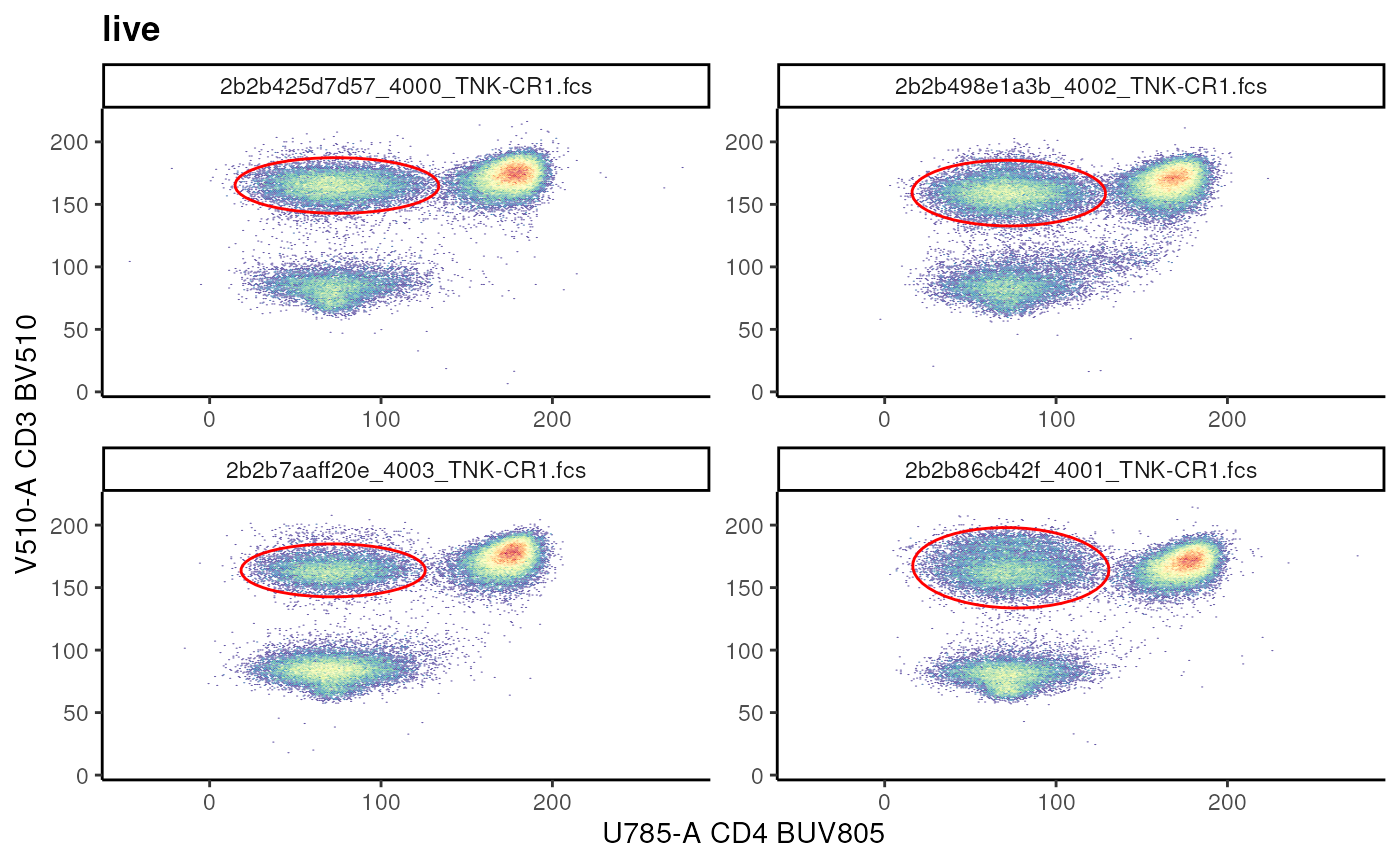

Exercise

How would you add a gate called CD4+ T Cells defined as: CD4+ and CD3+?
Hint: Use the visualization above to provide an appropriate target.
gating_args above indicates K = 3, quantile = 0.9, plot = FALSE. Try running the code block by indicating plot = TRUE. What is the outcome? How can you run this code block again? Hint: try running help.search(pattern = "remove gating").

Quad gate

When there are population(s) of interest in all 4 quadrants, it is useful to estimate a quadrant gate using gate_quad_sequential. Note: Pay attention to alias and pop arguments!

# plot subsets
t_subsets <- ggcyto(
  gs,
  subset = "CD3+",
  aes(x = "CD45RA", y = "CCR7")
)+
geom_hex(bins = 256)+
facet_wrap(~name)

# visualize
# t_subsets

# estimate and add
gs_add_gating_method(
  gs,
  alias = "*",
  pop = "+/-+/-",
  parent = "CD3+",
  dims = "CD45RA,CCR7",
  gating_method = "gate_quad_sequential",
  gating_args = list(
    gFunc = "mindensity"
  ),
  collapseDataForGating = TRUE
)

Exercise

How would you confirm that the attached gates have correct boundaries? Hint: Refer to the section on visualization.
How would you remove the gates attached by gs_add_gating_method? Hint: Try running help(gs_add_gating_method) and read the details.
gs_remove_gating_method reverses the the results of gs_add_gating_method in a step wise manner.
Are there other arguments for gs_add_gating_method? How can you use them?

Note: gs_add_gating_method keeps a history of the calls made. If you reload a previously saved GatingSet via load_gs to work on, start with a clean history using gs_add_gating_method_init(gs) so that errors do not arise.

Explicit construction of gates

Suppose you would like to add a gate that has a particular shape or range that cannot be easily estimated using the automatic estimation approaches above. In this case, you could programmatically define a gate by either providing ranges, coordinates, or logical statements as demonstrated below.

Rectangular gate

As the name suggests, we can explicitly define a rectangular gate by by defining a matrix where the columns are the ranges for markers in x-axis and y-axis. Only 1 dimension can also be provided. In this scenario, the constructed gate filter the events marginated over the dimension provided.

## Example of rectangleGate
cd3_vis <- ggcyto(
  gs, subset = "root", aes(x = "CD3", y = "CD56")
)+
  geom_hex(bins = 256)+
  facet_wrap(~name)

# before
# cd3_vis

# using rectangle gate to add T cell gate
cd3_rectangle <- matrix(
  c(140, 205, 0, 200),
  nrow = 2,
  ncol = 2,
  byrow = F,
  dimnames = list(
    c("min", "max"), # rownames
    c("V510-A","U570-A") # colnames are channel names
  )
) 
cd3_rectangle_gate <- rectangleGate(
  .gate = cd3_rectangle,
  filterId = "CD3+ T cells"
)
cd3_vis+geom_gate(cd3_rectangle_gate)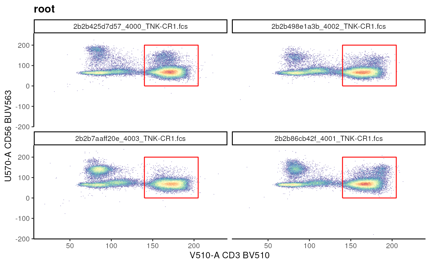

When a single dimension is provided:

# provide the range
cd3_range <- matrix(data = c(140,200))
# set the column name to the required channel
colnames(cd3_range) <- "V510-A"

# construct gate
cd3_range_gate <- rectangleGate(
  .gate = cd3_range,
  filterId = "CD3+ Range"
) 

cd3_vis + geom_gate(cd3_range_gate)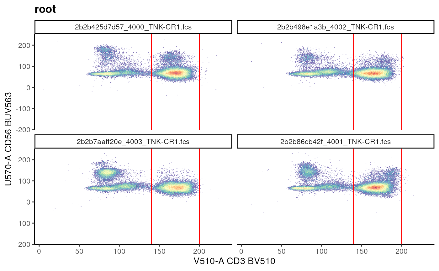

To add this gate we call gs_pop_add like so:

gs_pop_add(
  gs,
  parent = "live",
  gate = cd3_range_gate
)

## [1] 13

Each call to gs_pop_add requires a recompute(gs) call.

Exercise

Try to run the following code:

no_recompute <- ggcyto(gs, 
       subset = "CD3+ Range",
       aes(x = "CD3", y = "CD4"))+
  geom_hex(bins = 256)
no_recompute

Why do you get an error?

While gs_add_pop attaches the gates to the GatingSet, the index of the filtered events are not calculated until you call recompute.

Polygon gate

Similar to Rectangular gate we can define a Polygon gate by generating a matrix of vertices.

Here, each row of the matrix is the coordinate for a vertex and the columns are the channels.

## Example of polygonGate
nkt_vis <- ggcyto(gs, subset = "root",
                  aes(x = "CD1d", y = "CD3"))+ # fuzzy matching of marker names
  geom_hex(bins = 256)+
  facet_wrap(~name)

## Warning in getChannelMarker(frm, dim): CD1d is partially matched with
## R670-ACD1d:PBS57 tet APC

# visualize
# nkt_vis

# define coordinates
## coordinates are based on visualization!
nkt_poly <- matrix(
  c(
    115,140, # are arranged as x,y pair
    150,150,
    150,180,
    200,180,
    200,140 
  ), 
  ncol = 2,
  byrow = T, # indicates that add as x,y pair
  dimnames = list(
    NULL, # rownames have no meaning in polygonGates
    c("R670-A","V510-A") # colnames are channel names
  ) 
)

# create a gate
nkt_poly_gate <- polygonGate(
  nkt_poly,
  filterId = "NKT cells"
)
# visualize
nkt_vis + geom_gate(nkt_poly_gate)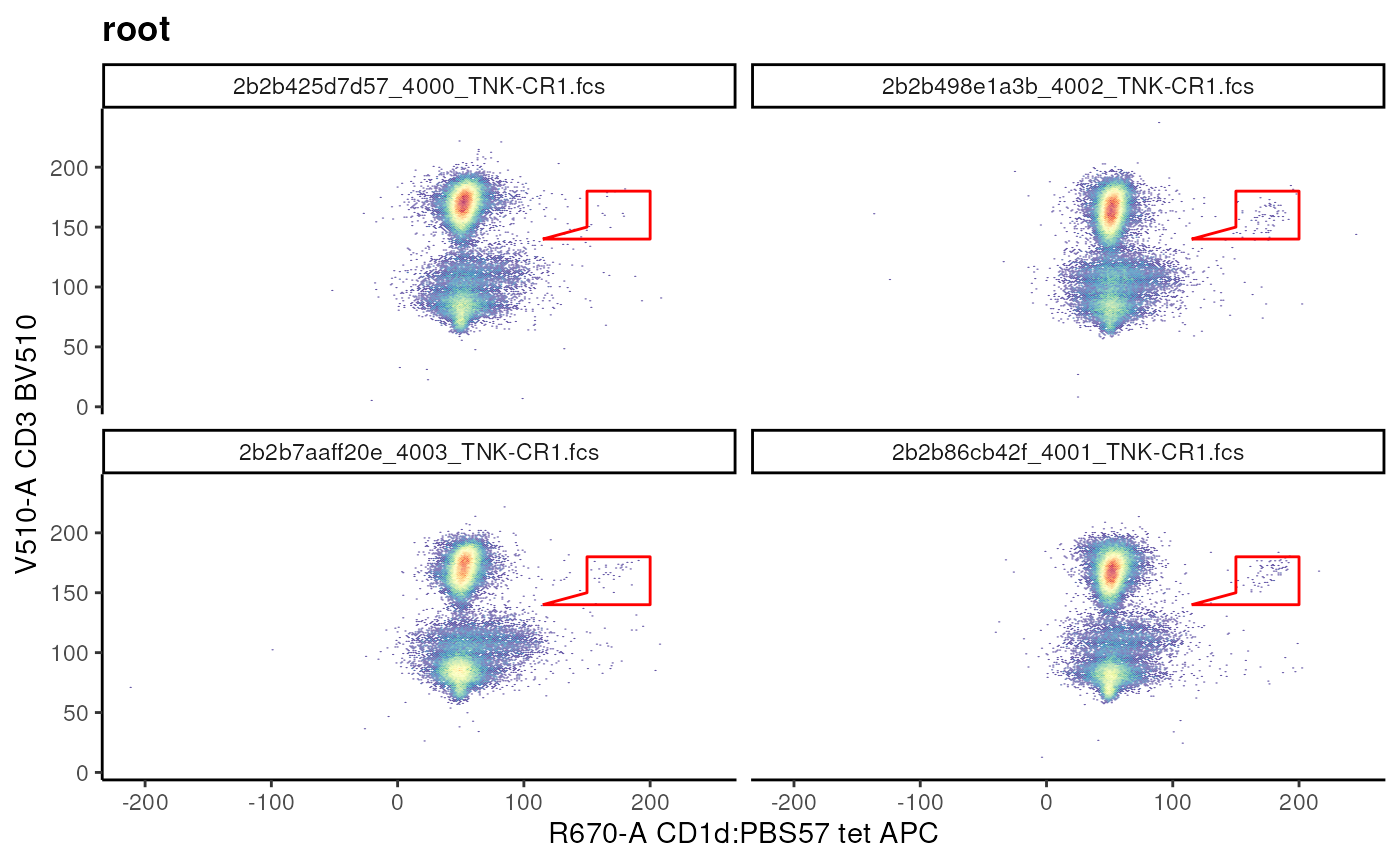

Editing a gate after construction is straight forward.

# move up and scale
nkt_poly_gate_scale <- flowCore::transform_gate(
  nkt_poly_gate, # gate object
  dx = 1, # which dimension to shift and by how much
                                        # dy = 1,
                                        # scale = 2 # scales both dimensions equally
  scale = c(1.05,1.05) # individually scale each dimension
)
nkt_vis+geom_gate(nkt_poly_gate_scale)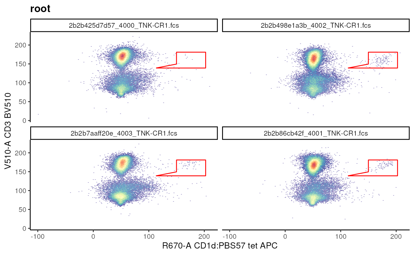

Exercise

Construct a new Rectangular gate that can be used to filter CD4- CD3+ population. Hint: Visualize the data and then define the best ranges.
How would you rotate this gate? Hint: try running help(flowCore::transform_gate).
Think back to the CD3+ gate we created using gs_add_gating_method, how would you edit it? Hint: try running help.search("get or set gate").

Boolean Gates

We can use booleanFilter to simply negate a gated population! The resulting filter does not have a geometric representation.

# add not MAIT gate
## Example of booleanFilter
not_mait <- booleanFilter(`!MAIT Cells`, filterId = "not_MAIT")

# add Boolean gate
gs_pop_add(
  gs, 
  not_mait, 
  parent = "live"
)

## [1] 14

recompute(gs)

# visualize
t_cell_vis+
  geom_overlay(
    gs_pop_get_data(gs, y = "not_MAIT"),
    size = 0.3, 
    colour = "red"
  )

Note: We are also able to combine multiple gates to generate a booleanFilter.

Let’s create by combining not_MAIT and MAIT Cells

# using an OR ('|') operator
all_cells <- booleanFilter(
  `not_MAIT|MAIT Cells`,
  filterId = "All"
)
# add population
gs_pop_add(gs, all_cells, parent = "live")
recompute(gs)

Exercise

How would you create a booleanFilter that only filters out naive T cells defined as CD45RA+CCR7+? Can you visualize the result?
How would you remove the gate called All?
How would you remove an attached gate? Is recompute required after removal of a gate?
What happens if you remove a parent gate?

Visualizing the Gating Hierachy

We have been creating and adding many gates to our GatingSet. A useful way to visualize all the gates and their relationship is by plotting the gating Hierarchy as a tree. This gives us an immediate summary of what nodes are present in our GatingSet.

# plot the gating tree
plot(gs, bool = TRUE)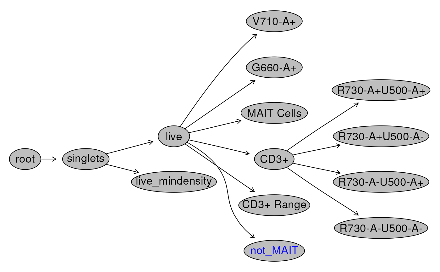

Another useful approach is to visualize the gated data, with gates that we have generated. See the section of visualization for more.

# visualize the full gating hierarchy
autoplot(
  gs[[1]],
  bins = 256, 
  bool = TRUE)+
  ggcyto_par_set(limits = "data") # set data range to be determined by data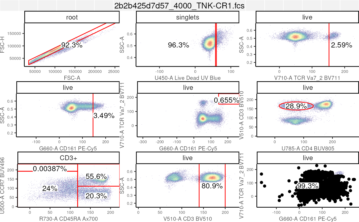

Saving your work

Finally, we save your GatingSet. The GatingSet can be loaded back into R using load_gs("path/to/a/folder").

# save your work
save_gs(gs, path = "path/to/a/folder")

Conclusion

In this section, we spent some time identifying various types of gates that are available in cytoverse. As well, we demonstrated how to programmatically create such gates, either manually (i.e. by defining ranges or vertices) or in a semi-automated and data driven manner.

Next, we go over methods to extract the gated data.

The (Optional) Part 3 goes over how users can leverage a gatingTemplate to generate gates as we have done here, but with minimal scripting. It is worth noting that while the use gatingTemplate minimizes scripting, it does not compromise on reproducibility!

Lastly, we also made ample use of the ggcyto library in order to generate visualizations that helped in QC’ing the data and the gates that we generated. We will go over ggcyto in more detail in Visualizations.

Background

GatingSet and GatingHeirarchy

Creating a GatingSet

Exercise

Exercise

A note about GatingHierarchy

Exercise

Adding gates and building a hierarchy

Automatic estimation of gates

Singlets gate

Estimating cutpoint and ranges using gate_quantile and gate_mindensity2

Estimating an Ellipsoid gate

Exercise

Quad gate

Exercise

Explicit construction of gates

Rectangular gate

Exercise

Polygon gate

Exercise

Boolean Gates

Exercise

Visualizing the Gating Hierachy

Saving your work

Conclusion

Creating a `GatingSet`

A note about `GatingHierarchy`

Estimating cutpoint and ranges using `gate_quantile` and `gate_mindensity2`