Importing and Basics of working with FCS files

Introduction

Flow cytometry data (regardless of the type of instrument used) is generally saved as a .fcs file. This file is populated with raw data, fluorescence intensity (for optics based technologies) and abundance (for mass cytrometry), as well as various metadata including: user id, instrument id, dynamic range of instrument, etc. It is important to be able to interact with and manipulate the .fcs file as it gives the users/analysts fine grain control!

Installing/loading required libraries

In the workshop, all the cytoverse packages are included in the instance you launched on the Bioconductor Workshop Galaxy, and the docker image this uses will remain available indefinitely (see the README.md for details). That said, if you want to install and use cytoverse packages outside of docker, the standard Bioconductor tooling works:

install.packages("BiocManager")
BiocManager::install("cytolib")
BiocManager::install("flowCore")
BiocManager::install("flowWorkspace")
BiocManager::install("ggcyto")
BiocManager::install("openCyto")
BiocManager::install("flowStats")
BiocManager::install("CytoML")

For the moment, we only need to load flowCore and flowWorkspace.

library(flowCore)
library(flowWorkspace)
library(CytoverseBioc2023)
cache_workshop_data()

FlowRepository workshop data

In this cytoverse workshop we will demonstrate the use of cytoverse packages to analyse publicly available datasets hosted on FlowRepository. The first dataset FR-FCM-Z5PC contains FCS files from a study assessing the post recovery immune phenotypes from patients infected with COVID-19. We are using a subset of the FCS files. The second dataset FR-FCM-ZZ36 contains FCS files for OMIP-018, a study designed to phenotype T cells for expression of various chemokine receptors.

The data required for this workshop, including subsets extracted from the FlowRepository datasets are made available locally in a file cache by running cache_workshop_data().

`cytoverse` data structures for .fcs files

There are four main data structures that represent flow cytometry data in cytoverse: cytoframe, cytoset, GatingHierarchy and GatingSet.

cytoframe: a single .fcs file,
cytoset: a list like object that can store multiple .fcs files,
GatingHierarchy: a list like object that allows building and attaching gates and filter to a cytoframe
GatingSet: a list like object that allows building and attaching gates and filter to a cytoset

Some of these have overlapping functionality, and we’ll eventually explain when you would prefer one data structure to another as we continue through this workshop.

Note:

There are additional legacy data structures called flowFrame and flowSet in cytoverse that are analogous to cytoframe and cytoset in function. We will not use these data structures in this workshop.

Reading in FCS files

There are two preferred approaches to read in .fcs file(s) into R:

Read in individual .fcs files as cytoframe,
Read in a set of .fcs files as cytoset,

(Additionally, you can read a workspace generated with another tool, such as FlowJo, using the CytoML package.)

The function load_cytoframe_from_fcs is used to read in individual file as a cytoframe object.

Normally, you might download a folder with a set of FCS files and interact with that. For instance,

For technical reasons, we can’t easily distribute the .fcs files in this way for this workshop, but instead reference them through a file cache. This cache is essentially a set of folders, however, and we specify which files we want in it with get_workshop_data.

If you want to explore it, you can examine it with BiocFileCache::bfcinfo(CytoverseBioc2023:::.get_cache()) or you can see some additional details below:

# structure of cached workshop data
data/
├── FlowRepository_FR-FCM-ZZ36_files
│   ├── Compensation Controls_APC Stained Control.fcs
│   ├── Compensation Controls_APC-Cy7 Stained Control.fcs
│   ├── Compensation Controls_Alexa Fluor 405 Stained Control.fcs
│   ├── Compensation Controls_Alexa Fluor 430 Stained Control.fcs
│   ├── Compensation Controls_Alexa Fluor 488 Stained Control.fcs
│   ├── Compensation Controls_PE Stained Control.fcs
│   ├── Compensation Controls_PE-Cy5 Stained Control.fcs
│   ├── Compensation Controls_PE-Cy5-5 Stained Control.fcs
│   ├── Compensation Controls_PE-Cy7 Stained Control.fcs
│   ├── Compensation Controls_PE-Texas Red Stained Control.fcs
│   ├── Compensation Controls_PerCP-Cy5-5 Stained Control.fcs
│   ├── Compensation Controls_Qdot 605 Stained Control.fcs
│   ├── Compensation Controls_Qdot 655 Stained Control.fcs
│   ├── Compensation Controls_Qdot 800 Stained Control.fcs
│   ├── Compensation Controls_Unstained Control.fcs
│   ├── control_files.csv
│   ├── pbmc_luca.fcs
│   └── spillover_from_FJ.csv
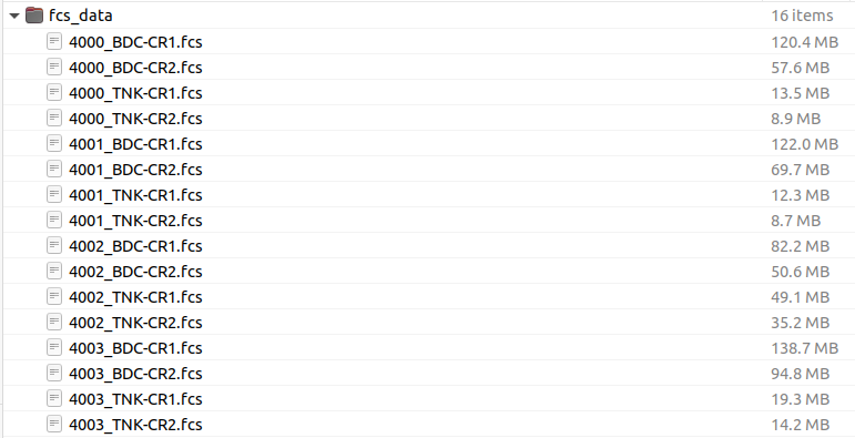
├── fcs_data
│   ├── 4000_BDC-CR1.fcs
│   ├── 4000_TNK-CR1.fcs
│   ├── 4001_BDC-CR1.fcs
│   ├── 4001_TNK-CR1.fcs
│   ├── 4002_TNK-CR1.fcs
│   └── 4003_TNK-CR1.fcs
├── fj_wsp
│   ├── 210224_BDC_CR1_analysis_template.wsp
│   ├── 210224_BDC_CR2_analysis_template.wsp
│   ├── 210224_TNK-CR2_analysis_template.wsp
│   ├── 210520_TNK-CR1_analysis_template.wsp
│   ├── analysis_copy.wsp
│   └── fj_transform.gz
├── gating_template
│   └── gating_template_TNK.csv
└── metadata
    └── 220115_Demographics_for_raw_data_upload.csv

Throughout this workshop we will use get_workshop_data() to return information about the location of the cached files so that they can be easily accessed for downstream analyses. get_workshop_data() returns a tibble containing information about the cached data including the path to the requested file(s) as indicated in the rpath variable.

# get location of cached data
cache_info <- get_workshop_data("gating_template_TNK.csv")
colnames(cache_info)

##  [1] "rid"                "rname"              "create_time"       
##  [4] "access_time"        "rpath"              "rtype"             
##  [7] "fpath"              "last_modified_time" "etag"              
## [10] "expires"

cf <- load_cytoframe_from_fcs(
  get_workshop_data(
    "data/fcs_data/4000_TNK-CR1.fcs"
  )$rpath
)

# a cytoframe object
cf

## cytoframe object '2b2b425d7d57_4000_TNK-CR1.fcs'
## with 102015 cells and 33 observables:
##                   name            desc     range  minRange  maxRange
## $P1              FSC-A              NA    262143    0.0000    262143
## $P2              FSC-H              NA    262143    0.0000    262143
## $P3              SSC-A              NA    262143    0.0000    262143
## $P4             B515-A    TCR Vd1 FITC    262143  -15.6344    262143
## $P5             B610-A     CD127 BB630    262143  -28.6509    262143
## ...                ...             ...       ...       ...       ...
## $P29            V710-A TCR Va7_2 BV711    262143  -56.8302    262143
## $P30            V750-A    CX3CR1 BV750    262143  -94.4459    262143
## $P31            V785-A      CD27 BV786    262143  -68.9282    262143
## $P32 remove_from_FS_FM              QC    262143    0.0000    262143
## $P33              Time              NA        93    0.0000        93
## 327 keywords are stored in the 'description' slot
## row names(0):

The cytoframe object has 3 slots where various data is stored.

exprs(cf) stores the expression matrix (i.e. the collected data),
parameters(cf) stores information pertaining to channels: channel name, marker description,and data ranges as an AnnotatedDataFrame,
keyword(cf) stores additional information extracted from the .fcs file header. The file header follow ISAC guidelines. Visit here for more information.

Working with `cytoframe` objects

A few useful definitions that help us get oriented with the underlying data in the cytoframe object.

Channels: Instrument derived labels of various parameters that were measured. Channels are the column names of the cytoframe. Any data generated from the same instrument will have the same (similar) Channel names.
Markers: User provided labels for various parameters that were measured. For example: Channel name: B710-A, Marker name: CD3 (in cf). Marker names are set by the users and may not be unique across experiments/users. Not all channels are markers – some are physical parameters such as the forward scatter or side scatter. These channels will have their marker names set to NA.
Expression: Measured values. A matrix where every row is an event (frequently a cell) and every column is a channel.

Working with a cytoframe object is very similar to working with a data.frame in R, where a “row” is a cell and a “column” is a channel. In particular, subsetting with square brackets cf[i,j] or cf$ works as you might hope. An important difference, however, is that unlike most other functions in R, the subset and assignment operations DO NOT create a new copy of the data but simply provides an updated “view” of the data. Because this is quite unlike the rest of R, we will perseverate on this point.

Examples

Accessing parameter summary and metadata

Summary of measured parameters.

# parameters
parameters(cf) |> pData() # show as a dataframe

##                   name               desc  range  minRange maxRange
## $P1              FSC-A               <NA> 262143   0.00000   262143
## $P2              FSC-H               <NA> 262143   0.00000   262143
## $P3              SSC-A               <NA> 262143   0.00000   262143
## $P4             B515-A       TCR Vd1 FITC 262143 -15.63437   262143
## $P5             B610-A        CD127 BB630 262143 -28.65089   262143
## $P6             B660-A          PD1 BB660 262143 -27.92371   262143
## $P7             B710-A         CD16 BB700 262143 -59.19245   262143
## $P8             B780-A        CXCR5 BB790 262143 -43.04906   262143
## $P9             G575-A         TCR Vg9 PE 262143 -56.83300   262143
## $P10            G610-A   TCR Vd2 PE-CF594 262143 -41.95899   262143
## $P11            G660-A       CD161 PE-Cy5 262143 -80.99514   262143
## $P12            G710-A     HLA-DR PE-Cy55 262143 -18.96598   262143
## $P13            G780-A        CCR1 PE-Cy7 262143 -36.50302   262143
## $P14            R670-A CD1d:PBS57 tet APC 262143 -29.70142   262143
## $P15            R730-A       CD45RA Ax700 262143 -25.40188   262143
## $P16            R780-A   XCR1 APC-Fire750 262143 -44.47800   262143
## $P17            U390-A        CCR3 BUV395 262143 -34.30737   262143
## $P18            U450-A  Live Dead UV Blue 262143 -33.85764   262143
## $P19            U500-A        CCR7 BUV496 262143 -41.69565   262143
## $P20            U570-A        CD56 BUV563 262143 -55.82978   262143
## $P21            U660-A        CD39 BUV661 262143 -40.15375   262143
## $P22            U740-A        CD95 BUV737 262143 -61.74041   262143
## $P23            U785-A         CD4 BUV805 262143 -80.50024   262143
## $P24            V450-A         CCR2 BV421 262143 -15.04627   262143
## $P25            V510-A          CD3 BV510 262143 -47.88375   262143
## $P26            V570-A         CD8a BV570 262143 -26.94096   262143
## $P27            V605-A         CD38 BV605 262143 -24.60269   262143
## $P28            V655-A         CCR5 BV650 262143 -29.68589   262143
## $P29            V710-A    TCR Va7_2 BV711 262143 -56.83018   262143
## $P30            V750-A       CX3CR1 BV750 262143 -94.44585   262143
## $P31            V785-A         CD27 BV786 262143 -68.92819   262143
## $P32 remove_from_FS_FM                 QC 262143   0.00000   262143
## $P33              Time               <NA>     93   0.00000       93

Various metadata present in the .fcs files.

# keywords
keyword(cf) |> head(10) # only show the first 10

## $FCSversion
## [1] "3"
## 
## $`$FIL`
## [1] "4000_TNK-CR1.fcs"
## 
## $`$TOT`
## [1] "102015"
## 
## $`$PAR`
## [1] "33"
## 
## $`$BYTEORD`
## [1] "4,3,2,1"
## 
## $`$DATATYPE`
## [1] "F"
## 
## $FJ_FCS_VERSION
## [1] "3"
## 
## $`$BEGINANALYSIS`
## [1] "0"
## 
## $`$BEGINSTEXT`
## [1] "0"
## 
## $`$BTIM`
## [1] "12:36:14"

Channels, Expression, and Subsets

# channels
colnames(cf)

##  [1] "FSC-A"             "FSC-H"             "SSC-A"            
##  [4] "B515-A"            "B610-A"            "B660-A"           
##  [7] "B710-A"            "B780-A"            "G575-A"           
## [10] "G610-A"            "G660-A"            "G710-A"           
## [13] "G780-A"            "R670-A"            "R730-A"           
## [16] "R780-A"            "U390-A"            "U450-A"           
## [19] "U500-A"            "U570-A"            "U660-A"           
## [22] "U740-A"            "U785-A"            "V450-A"           
## [25] "V510-A"            "V570-A"            "V605-A"           
## [28] "V655-A"            "V710-A"            "V750-A"           
## [31] "V785-A"            "remove_from_FS_FM" "Time"

# markernames
markernames(cf)

##               B515-A               B610-A               B660-A 
##       "TCR Vd1 FITC"        "CD127 BB630"          "PD1 BB660" 
##               B710-A               B780-A               G575-A 
##         "CD16 BB700"        "CXCR5 BB790"         "TCR Vg9 PE" 
##               G610-A               G660-A               G710-A 
##   "TCR Vd2 PE-CF594"       "CD161 PE-Cy5"     "HLA-DR PE-Cy55" 
##               G780-A               R670-A               R730-A 
##        "CCR1 PE-Cy7" "CD1d:PBS57 tet APC"       "CD45RA Ax700" 
##               R780-A               U390-A               U450-A 
##   "XCR1 APC-Fire750"        "CCR3 BUV395"  "Live Dead UV Blue" 
##               U500-A               U570-A               U660-A 
##        "CCR7 BUV496"        "CD56 BUV563"        "CD39 BUV661" 
##               U740-A               U785-A               V450-A 
##        "CD95 BUV737"         "CD4 BUV805"         "CCR2 BV421" 
##               V510-A               V570-A               V605-A 
##          "CD3 BV510"         "CD8a BV570"         "CD38 BV605" 
##               V655-A               V710-A               V750-A 
##         "CCR5 BV650"    "TCR Va7_2 BV711"       "CX3CR1 BV750" 
##               V785-A    remove_from_FS_FM 
##         "CD27 BV786"                 "QC"

# instrument channel ranges
range(cf, type = "instrument")

##      FSC-A  FSC-H  SSC-A       B515-A       B610-A       B660-A       B710-A
## min      0      0      0    -15.63437    -28.65089    -27.92371    -59.19245
## max 262143 262143 262143 262143.00000 262143.00000 262143.00000 262143.00000
##           B780-A     G575-A       G610-A       G660-A       G710-A       G780-A
## min    -43.04906    -56.833    -41.95899    -80.99514    -18.96598    -36.50302
## max 262143.00000 262143.000 262143.00000 262143.00000 262143.00000 262143.00000
##           R670-A       R730-A     R780-A       U390-A       U450-A       U500-A
## min    -29.70142    -25.40188    -44.478    -34.30737    -33.85764    -41.69565
## max 262143.00000 262143.00000 262143.000 262143.00000 262143.00000 262143.00000
##           U570-A       U660-A       U740-A       U785-A       V450-A
## min    -55.82978    -40.15375    -61.74041    -80.50024    -15.04627
## max 262143.00000 262143.00000 262143.00000 262143.00000 262143.00000
##           V510-A       V570-A       V605-A       V655-A       V710-A
## min    -47.88375    -26.94096    -24.60269    -29.68589    -56.83018
## max 262143.00000 262143.00000 262143.00000 262143.00000 262143.00000
##           V750-A       V785-A remove_from_FS_FM Time
## min    -94.44585    -68.92819                 0    0
## max 262143.00000 262143.00000            262143   93

# expression
exprs(cf)[1:5, 1:5]

##          FSC-A    FSC-H    SSC-A   B515-A    B610-A
## [1,] 103038.81 88791.99 519.6562 345.1194 2290.9805
## [2,]  94411.01 79966.73 926.6454 327.2972 2667.8779
## [3,]  93067.27 76786.17 917.7739 335.5514 2857.0173
## [4,]  94072.62 87279.86 337.3925 252.7754  895.4494
## [5,] 102544.66 81934.16 626.8440 760.3972 2160.2334

# number of events
nrow(cf)

## [1] 102015

# number of channels 
ncol(cf)

## [1] 33

Notice that there is a correspondence between channels, markers, and the expression matrix. i.e. the names of the named vector markernames(cf) are a subset of the columns of the expression matrix exprs(cf) as well as the columns of the cytoframe.

# interested marker: CD4
# easy to find which channel is mapped to CD4
CD4_chan <- flowCore::getChannelMarker(
  frm = cf,
  name = "CD4"
)$name

# inspect CD4_chan
CD4_chan

## [1] "U785-A"

# extract expression of cd4
e_cd4 <- exprs(cf[, CD4_chan])
head(e_cd4)

##         U785-A
## [1,] 2191.3669
## [2,] 2586.0300
## [3,] 3177.3501
## [4,]  486.9400
## [5,]  691.0447
## [6,]  556.0515

# subset cytorame by column
s_cf <- cf[, CD4_chan]
s_cf

## cytoframe object '2b2b425d7d57_4000_TNK-CR1.fcs'
## with 102015 cells and 1 observables:
##        name       desc     range  minRange  maxRange
## $P23 U785-A CD4 BUV805    262143  -80.5002    262143
## 327 keywords are stored in the 'description' slot
## row names(0):
## cytoframe has been subsetted and can be realized through 'realize_view()'.

# subset cytoframe by row
s2_cf <- cf[1:100, ]
s2_cf

## cytoframe object '2b2b425d7d57_4000_TNK-CR1.fcs'
## with 100 cells and 33 observables:
##                   name            desc     range  minRange  maxRange
## $P1              FSC-A              NA    262143    0.0000    262143
## $P2              FSC-H              NA    262143    0.0000    262143
## $P3              SSC-A              NA    262143    0.0000    262143
## $P4             B515-A    TCR Vd1 FITC    262143  -15.6344    262143
## $P5             B610-A     CD127 BB630    262143  -28.6509    262143
## ...                ...             ...       ...       ...       ...
## $P29            V710-A TCR Va7_2 BV711    262143  -56.8302    262143
## $P30            V750-A    CX3CR1 BV750    262143  -94.4459    262143
## $P31            V785-A      CD27 BV786    262143  -68.9282    262143
## $P32 remove_from_FS_FM              QC    262143    0.0000    262143
## $P33              Time              NA        93    0.0000        93
## 327 keywords are stored in the 'description' slot
## row names(0):
## cytoframe has been subsetted and can be realized through 'realize_view()'.

Notice that the subset (<- [) operation can be applied directly to the cytoframe object so that information regarding the file is preserved. Also, as indicated above, these operations provide an aliased view of the data without creating a copy.

Below, we show examples of how to manipulate the cytoframe object and create a copy using realize_view():

# create a new markername
new_name <- c("U785-A" = "test")

# create a new cytoframe subset
cf_sub <- cf[1:150, ] |> realize_view() # realize_view creates a new cytoframe, distinct from the original

# old markernames
markernames(cf_sub)

##               B515-A               B610-A               B660-A 
##       "TCR Vd1 FITC"        "CD127 BB630"          "PD1 BB660" 
##               B710-A               B780-A               G575-A 
##         "CD16 BB700"        "CXCR5 BB790"         "TCR Vg9 PE" 
##               G610-A               G660-A               G710-A 
##   "TCR Vd2 PE-CF594"       "CD161 PE-Cy5"     "HLA-DR PE-Cy55" 
##               G780-A               R670-A               R730-A 
##        "CCR1 PE-Cy7" "CD1d:PBS57 tet APC"       "CD45RA Ax700" 
##               R780-A               U390-A               U450-A 
##   "XCR1 APC-Fire750"        "CCR3 BUV395"  "Live Dead UV Blue" 
##               U500-A               U570-A               U660-A 
##        "CCR7 BUV496"        "CD56 BUV563"        "CD39 BUV661" 
##               U740-A               U785-A               V450-A 
##        "CD95 BUV737"         "CD4 BUV805"         "CCR2 BV421" 
##               V510-A               V570-A               V605-A 
##          "CD3 BV510"         "CD8a BV570"         "CD38 BV605" 
##               V655-A               V710-A               V750-A 
##         "CCR5 BV650"    "TCR Va7_2 BV711"       "CX3CR1 BV750" 
##               V785-A    remove_from_FS_FM 
##         "CD27 BV786"                 "QC"

# set new markername
markernames(cf_sub) <- new_name
markernames(cf_sub)

##               B515-A               B610-A               B660-A 
##       "TCR Vd1 FITC"        "CD127 BB630"          "PD1 BB660" 
##               B710-A               B780-A               G575-A 
##         "CD16 BB700"        "CXCR5 BB790"         "TCR Vg9 PE" 
##               G610-A               G660-A               G710-A 
##   "TCR Vd2 PE-CF594"       "CD161 PE-Cy5"     "HLA-DR PE-Cy55" 
##               G780-A               R670-A               R730-A 
##        "CCR1 PE-Cy7" "CD1d:PBS57 tet APC"       "CD45RA Ax700" 
##               R780-A               U390-A               U450-A 
##   "XCR1 APC-Fire750"        "CCR3 BUV395"  "Live Dead UV Blue" 
##               U500-A               U570-A               U660-A 
##        "CCR7 BUV496"        "CD56 BUV563"        "CD39 BUV661" 
##               U740-A               U785-A               V450-A 
##        "CD95 BUV737"               "test"         "CCR2 BV421" 
##               V510-A               V570-A               V605-A 
##          "CD3 BV510"         "CD8a BV570"         "CD38 BV605" 
##               V655-A               V710-A               V750-A 
##         "CCR5 BV650"    "TCR Va7_2 BV711"       "CX3CR1 BV750" 
##               V785-A    remove_from_FS_FM 
##         "CD27 BV786"                 "QC"

# manipulating expression values
# notice the data range 
range(cf_sub[, "U785-A"])

##           U785-A
## min    -80.50024
## max 262143.00000

# visualise original channel ditribution
plot(
  density(
    exprs(cf_sub[, "U785-A"])
  ),
  main = "U785-A"
)

# asinh transform
exprs(cf_sub)[, "U785-A"] <- asinh(exprs(cf_sub)[, "U785-A"])

# notice the data range after transformation
range(
  cf_sub[, "U785-A"],
  type = "instrument"
)

##           U785-A
## min    -80.50024
## max 262143.00000

# visualise channel distribution
plot(
  density(
    exprs(cf_sub[, "U785-A"])
  ),
  main = "U785-A"
)

Notice that the data range summary was not updated when we used <- to change the underlying expression matrix. A good practice is to use transform function to transform the underlying expression matrix. Importantly, transform also updates the data range summary. Moreover, transform can also be used to add new columns to the cytoframe.

Note: We will go over transformations in a later section.

Exercise

Why is length(colnames(cf)) different than length(markernames(cf))?
How could you create a random downsample of 1000 cells from cf?
Make a scatter plot of the forward scatter (FSC-A) vs side scatter (SSC-A) of cf using a graphics package of your choice.

Reading in a set of FCS files as a `cytoset`

In a experimental sense, a single .fcs file is not very interesting, since this represents only a single sample. To draw any conclusions, we’ll want replicates. When there are a set of .fcs files they can be loaded into R either as a cytoset.

cytoset: A collection of .fcs files, preferably, but not necessarily from the same panel/experiment.

cs <- load_cytoset_from_fcs(
  files = get_workshop_data(
    path = "data/fcs_data/"
  )$rpath
)
cs

## A cytoset with 6 samples.
## 
##   column names:
##     FSC-A, FSC-H, SSC-A, B515-A, B610-A, B660-A, B710-A, B780-A, G575-A, G610-A, G660-A, G710-A, G780-A, R670-A, R730-A, R780-A, U390-A, U450-A, U500-A, U570-A, U660-A, U740-A, U785-A, V450-A, V510-A, V570-A, V605-A, V655-A, V710-A, V750-A, V785-A, remove_from_FS_FM, Time

A cytoset can also be indexed with square brackets cs[i,j], however now the row index i selects samples (individual FCS files) rather than cells. A cytoset also behaves like a list – a double bracket cs[[i]] selects a single sample as a cytoframe.

Generally, each FCS file replicate has unique metadata properties that can (and should) be supplied to the cytoset. These can be added after loading the cytoset by using pData(x) <- data.frame. The rownames of the data.frame must match the sampleNames of the cytoset.

# prior to providing metadata
pData(cs)

##                                                        name
## 2b2b446859e1_4000_BDC-CR1.fcs 2b2b446859e1_4000_BDC-CR1.fcs
## 2b2b425d7d57_4000_TNK-CR1.fcs 2b2b425d7d57_4000_TNK-CR1.fcs
## 2b2b935ef9e_4001_BDC-CR1.fcs   2b2b935ef9e_4001_BDC-CR1.fcs
## 2b2b86cb42f_4001_TNK-CR1.fcs   2b2b86cb42f_4001_TNK-CR1.fcs
## 2b2b498e1a3b_4002_TNK-CR1.fcs 2b2b498e1a3b_4002_TNK-CR1.fcs
## 2b2b7aaff20e_4003_TNK-CR1.fcs 2b2b7aaff20e_4003_TNK-CR1.fcs

# create metadata
metadata <- data.frame(
  Treatment = rep(c("Untreated","Treated"),
    length.out = length(cs)
  ),
  panel = ifelse(
    grepl(
      pattern = "TNK",
      x = sampleNames(cs)
    ),
    "T Cell Panel",
    "Myeloid Panel"
  )
)

Let’s see what happens when rownames do not match!

# try to add metadata  -- this leads to an error
pData(cs) <- metadata

## Error: Invalid input type, expected 'character' actual 'integer'

Now, we ensure that rownames of data.frame matches sampleNames of the cytoset.

# now it works
row.names(metadata) <- sampleNames(cs)
pData(cs) <- metadata
pData(cs)

##                               Treatment         panel
## 2b2b446859e1_4000_BDC-CR1.fcs Untreated Myeloid Panel
## 2b2b425d7d57_4000_TNK-CR1.fcs   Treated  T Cell Panel
## 2b2b935ef9e_4001_BDC-CR1.fcs  Untreated Myeloid Panel
## 2b2b86cb42f_4001_TNK-CR1.fcs    Treated  T Cell Panel
## 2b2b498e1a3b_4002_TNK-CR1.fcs Untreated  T Cell Panel
## 2b2b7aaff20e_4003_TNK-CR1.fcs   Treated  T Cell Panel

The benefit of having metadata is that we can use many of the sub-setting operations in a metadata specific manner.

This is much more convenient than going back and forth between the full set of files.

# subset by files that have myeloid staining panel without creating a copy of the data
cs_myeloid <- cs[pData(cs)[["panel"]] == "Myeloid Panel",]

cs_myeloid

## A cytoset with 2 samples.
## 
##   column names:
##     FSC-A, FSC-H, SSC-A, B515-A, B610-A, B660-A, B710-A, B780-A, G575-A, G610-A, G660-A, G710-A, G780-A, R670-A, R730-A, R780-A, U390-A, U450-A, U500-A, U570-A, U660-A, U740-A, U785-A, V450-A, V510-A, V570-A, V605-A, V655-A, V710-A, V750-A, V785-A, remove_from_FS_FM, Time

pData(cs_myeloid)

##                               Treatment         panel
## 2b2b446859e1_4000_BDC-CR1.fcs Untreated Myeloid Panel
## 2b2b935ef9e_4001_BDC-CR1.fcs  Untreated Myeloid Panel

Cytoset views and aliasing

Many of the sub-setting operation for cytoframe are also applicable for cytoset. Similar to cytoframe sub-setting operations only create a new “view” of the data. For a complete copy of the data, realize_view should be used.

Below is an example of cytoset sub-setting which also highlights how the operations performed on cytoset affects the underlying data.

# demonstrate how cs point to the same underlying data
range(cs[[1, "B515-A"]])

##          B515-A
## min   -110.3859
## max 262143.0000

# subset and show prior to transformation
cs_small <- cs[1]
range(cs_small[[1, "B515-A"]])

##          B515-A
## min   -110.3859
## max 262143.0000

# create a transformList
trans <- transformList("B515-A",asinh)

# transform
cs_small <- transform(cs_small,trans)

# after transformation
range(cs_small[[1, "B515-A"]])

##        B515-A
## min -5.397151
## max 13.169792

# whole cs 
range(cs[[1, "B515-A"]])

##        B515-A
## min -5.397151
## max 13.169792

As you see, the transformation was applied to a subset cs_small however the original cs was also altered highlighting that both objects were pointing to the same data. To confirm this, you can use cs_get_uri or cf_get_uri:

cs_get_uri(cs_small)

## [1] "/tmp/RtmpiZVSjq/be831c15-301d-475f-bd66-0a9250713415"

cs_get_uri(cs)

## [1] "/tmp/RtmpiZVSjq/be831c15-301d-475f-bd66-0a9250713415"

To perform a deep copy we can use realize_view()

# look at underlying expression
range(cs[[2, "B515-A"]])

##           B515-A
## min    -15.63437
## max 262143.00000

# subset and show prior to transformation
cs_small2 <- realize_view(cs[2])
range(cs_small2[[1, "B515-A"]])

##           B515-A
## min    -15.63437
## max 262143.00000

# create a transformList
trans <- transformList("B515-A",asinh)

# transform
cs_small2 <- transform(cs_small2,trans)

# after transformation
range(cs_small2[[1, "B515-A"]])

##       B515-A
## min -3.44364
## max 13.16979

# whole cs 
range(cs[[2, "B515-A"]])

##           B515-A
## min    -15.63437
## max 262143.00000

Notice that cs is left unchanged.

Exercise

Explain why the following code does not work as expected:

cf_log_trans <- cf
exprs(cf_log_trans) <- log2(exprs(cf))
plot(
  exprs(cf)[,"V510-A"], 
  exprs(cf_log_trans)[,"V510-A"],
  main = "Effect of log2 transformation on  V510-A (CD3)"
)

Adding additional .fcs files to `cytoset`

Lastly, we can also add additional .fcs files to a cytoset using cs_add_cytoframe.

# add to cytoset
cs_small <- realize_view(cs[1]) # cs[1] subsets cs into a cytoset while realize_view leads to a deep_copy into a new cytoset
cs_small

## A cytoset with 1 samples.
## 
##   column names:
##     FSC-A, FSC-H, SSC-A, B515-A, B610-A, B660-A, B710-A, B780-A, G575-A, G610-A, G660-A, G710-A, G780-A, R670-A, R730-A, R780-A, U390-A, U450-A, U500-A, U570-A, U660-A, U740-A, U785-A, V450-A, V510-A, V570-A, V605-A, V655-A, V710-A, V750-A, V785-A, remove_from_FS_FM, Time

# no need to assign back to cs_small, because this function operates by reference and returns NULL anyways.
cs_add_cytoframe(
  cs = cs_small,
  sn = "Sample Name",
  cf = cs[[3]]   # cs[[3]] results in a cytoframe
) 
cs_small

## A cytoset with 2 samples.
## 
##   column names:
##     FSC-A, FSC-H, SSC-A, B515-A, B610-A, B660-A, B710-A, B780-A, G575-A, G610-A, G660-A, G710-A, G780-A, R670-A, R730-A, R780-A, U390-A, U450-A, U500-A, U570-A, U660-A, U740-A, U785-A, V450-A, V510-A, V570-A, V605-A, V655-A, V710-A, V750-A, V785-A, remove_from_FS_FM, Time

From `cytoset` to `cytoframe`

It is possible that you may want to extract a cytoframe or extract all files as a list of cytoframe. We can either use [[ to directly grab a cytoframe or cytoset_to_list.

# extract a single cytoframe by using cs[[index/samplename]]
single_cf <- cs[[1]]

# convert to a list
list_of_cf <- cytoset_to_list(cs)

List like operation with `cytoset`

As indicated previously, a cytoset behaves like a list. To leverage this behaviour we can use fsApply to iterate through the samples in a cytoset. By default, output is attempted to be coerced to a single array like object. (Set simplify = FALSE to return another list.)

# getting number of rows (cells) of individual cytoframes
n_cell_events <- fsApply(cs, nrow)
n_cell_events

##                                 [,1]
## 2b2b446859e1_4000_BDC-CR1.fcs 912254
## 2b2b425d7d57_4000_TNK-CR1.fcs 102015
## 2b2b935ef9e_4001_BDC-CR1.fcs  924474
## 2b2b86cb42f_4001_TNK-CR1.fcs   92703
## 2b2b498e1a3b_4002_TNK-CR1.fcs 372224
## 2b2b7aaff20e_4003_TNK-CR1.fcs 146150

Exercises

How would you extract marker names that are stored within a the cytoset cs?
How would you create a cytoset from the object list_of_cf?

Saving your data

Saving your data is easy.

# save cytoframe
cf_write_disk(cf, "path/to/my_new_cf")

# save cytoset
save_cytoset(cs, path = "path/to/my/cs")

Loading it back is just as easy.

# load cytoframe
load_cytoframe("path/to/my_cf")

# load cytoset
load_cytoset("path/to/my/cs")

Conclusion

We went through multiple ways to import, interact with, and manipulate .fcs files using the cytoverse tools. It is important to note additional functionality, which we will not going to go over at this workshop for the sake of time, for further manipulation and even creation of .fcs files exist with the cytoverse. We encourage you to explore them further at your leisure by calling browseVignettes("flowWorkspace").

Introduction

Installing/loading required libraries

FlowRepository workshop data

cytoverse data structures for .fcs files

Reading in FCS files

Working with cytoframe objects

Examples

Accessing parameter summary and metadata

Channels, Expression, and Subsets

Exercise

Reading in a set of FCS files as a cytoset

Cytoset views and aliasing

Exercise

Adding additional .fcs files to cytoset

From cytoset to cytoframe

List like operation with cytoset

Exercises

Saving your data

Conclusion

`cytoverse` data structures for .fcs files

Working with `cytoframe` objects

Reading in a set of FCS files as a `cytoset`

Adding additional .fcs files to `cytoset`

From `cytoset` to `cytoframe`

List like operation with `cytoset`