Spillover, compensation, and Transformations
Source:vignettes/2_Spillover_transformation.Rmd
2_Spillover_transformation.RmdBackground
In this section, we aim to clarify the concept of Spillover, and the use of spillover matrix to correct for this. The last part of this section will deal with various transformations of the underlying expression data to aid in visualization and interpretation.
Spillover
Flow cytometers (optics based: spectral or non-spectral) collect fluorescent signal from a cell as result of a laser excitation. Briefly, cell type C has been labelled with a marker M that is conjugated to a fluorophore (F). F is excited by a laser resulting in fluorescence. While the fluorescence has a emission maxima, the emission profile of F can span many nanometers. The cytometer has a dedicated detector (channel) A to detect peak emission of F. However, due to the spread of the emission of F, some signal from F is also “spilled” onto detector B, a detector for a different fluorophore.
The image below provides a concrete example.
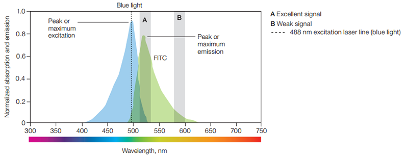
The spillover of signal onto secondary detector(s) is additive and can be easily recovered (more on this below).
Raw Signal in \(B = \text{Signal from FITC (spillover)} + \text{Signal from another (perhaps dedicated) fluorophore}.\)
FITC signal detected erroneously by secondary detectors can be estimated by a process of fluorescence compensation which requires a set of controls be present to calculate the spillover. These controls are called Single Colour Controls and are acquired prior to sample acquisition. The purpose of the single colour control is to estimate the amount of spillover of emission from fluorophore F onto non-primary detectors (detector B in the image above).
We note, but will not discuss further here that there are a class of more advanced fluorescence-based cytometers known as spectral flow cytometers. Spectral instruments require a different and more specialized procedure to perform compensation.
Importance of spillover correction
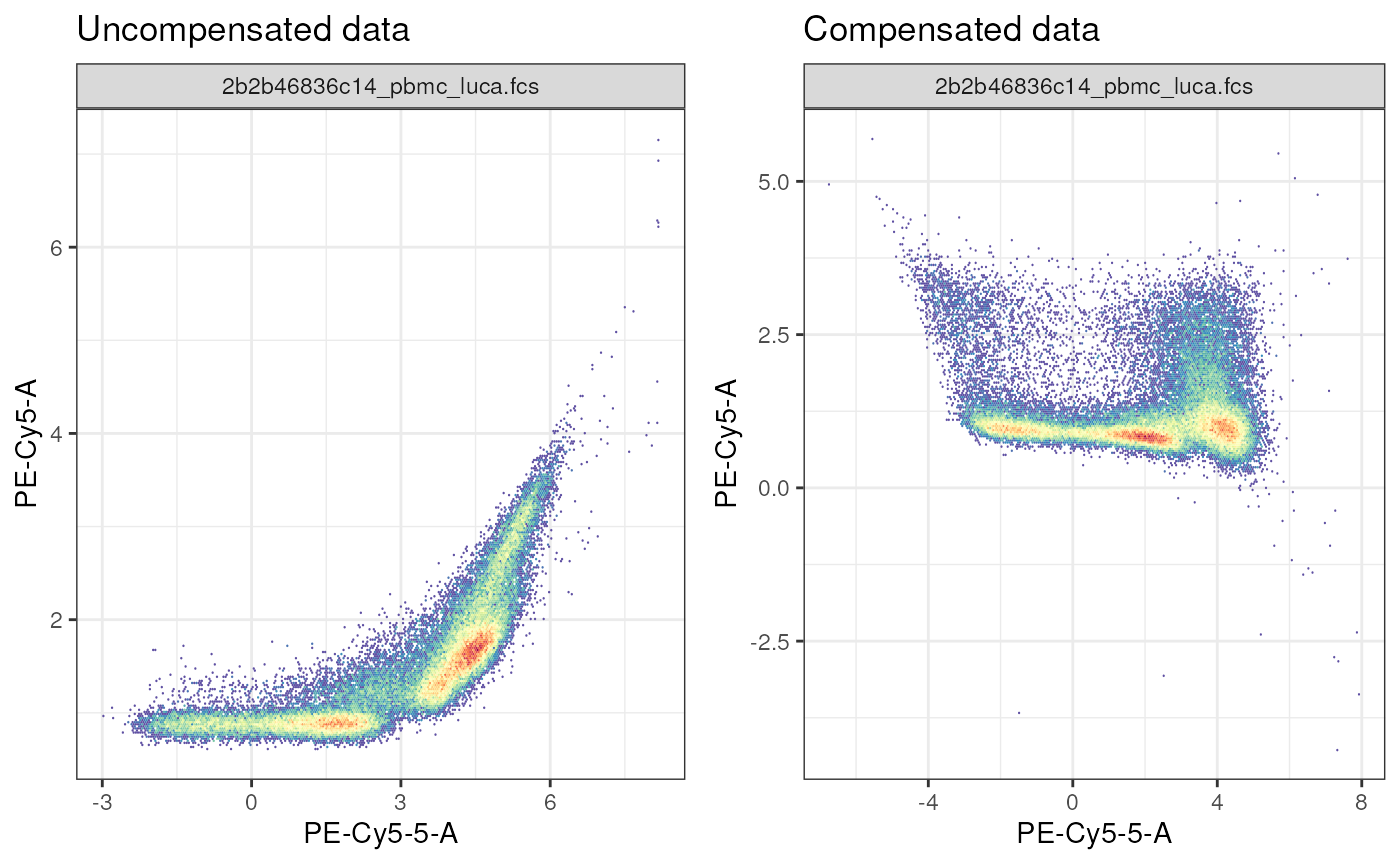
Let’s visualize the data to highlight the main issues related to
spillover. We will make use of the ggcyto library from the
cytoverse for this. We will dive into more details on the
usage of ggcyto in a later section, as well as the
“transformation” we are applying. For the moment, think of this
transformation as a glorified log-transform to visualize the fluorescent
signal that spans several orders of magnitude.
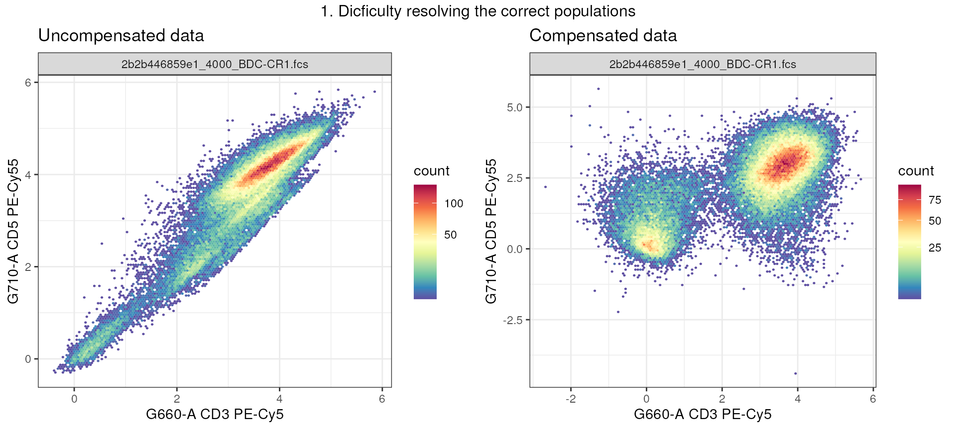
In example 1, the 2 fluorophores: PE-Cy5 and PE-Cy5.5 are spilling onto each other, making it impossible to resolve CD3+ (T cells) from non-T cells. However, after correcting for spillover (2nd plot), we see that two populations are visible in the G660-A CD3 PE-Cy5 channel.
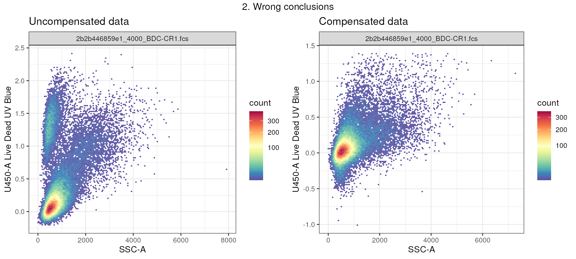
In example 2, we see a population of events that are positive of marker: Live Dead UV Blue. It would be tempting to exclude these events as this marker is used to identify dead cells. However, in correctly compensated data, we see that this population actually is not present, but rather was an artifact of another dye spilling onto the U450 channel!
Spillover matrix: What does it look like? Where do you find it? How can you use it?
Embedded with the .fcs file
In many cases, the spillover matrix (which is used to correct the
spillover) is attached to the .fcs files within
$SPILLOVER,SPILL,or SPILL
keywords. In cytoverse, we can check for
the presence of by using the function spillover(cf).
Example: absent or incorrect
For this example, we are using data from the following dataset FR-FCM-ZZ36. The data was published in this manuscript.
# absent spill
cf_absent <- load_cytoframe_from_fcs(
  get_workshop_data(
    "luca"
  )$rpath
)

# check spillover results
spillover(cf_absent)
## $SPILL
## Alexa Fluor 488-A PerCP-Cy5-5-A APC-A APC-Cy7-A Alexa Fluor 405-A
## [1,] 1 0 0 0 0
## [2,] 0 1 0 0 0
## [3,] 0 0 1 0 0
## [4,] 0 0 0 1 0
## [5,] 0 0 0 0 1
## [6,] 0 0 0 0 0
## [7,] 0 0 0 0 0
## [8,] 0 0 0 0 0
## [9,] 0 0 0 0 0
## [10,] 0 0 0 0 0
## [11,] 0 0 0 0 0
## [12,] 0 0 0 0 0
## [13,] 0 0 0 0 0
## [14,] 0 0 0 0 0
## Alexa Fluor 430-A Qdot 605-A Qdot 655-A Qdot 800-A PE-A PE-Texas Red-A
## [1,] 0 0 0 0 0 0
## [2,] 0 0 0 0 0 0
## [3,] 0 0 0 0 0 0
## [4,] 0 0 0 0 0 0
## [5,] 0 0 0 0 0 0
## [6,] 1 0 0 0 0 0
## [7,] 0 1 0 0 0 0
## [8,] 0 0 1 0 0 0
## [9,] 0 0 0 1 0 0
## [10,] 0 0 0 0 1 0
## [11,] 0 0 0 0 0 1
## [12,] 0 0 0 0 0 0
## [13,] 0 0 0 0 0 0
## [14,] 0 0 0 0 0 0
## PE-Cy5-A PE-Cy5-5-A PE-Cy7-A
## [1,] 0 0 0
## [2,] 0 0 0
## [3,] 0 0 0
## [4,] 0 0 0
## [5,] 0 0 0
## [6,] 0 0 0
## [7,] 0 0 0
## [8,] 0 0 0
## [9,] 0 0 0
## [10,] 0 0 0
## [11,] 0 0 0
## [12,] 1 0 0
## [13,] 0 1 0
## [14,] 0 0 1
##
## $spillover
## NULL
##
## $`$SPILLOVER`
## NULLNotice that there are 3 slots. Importantly, we notice a matrix within
$SPILL slot which has 1’s in the diagonal and 0’s
elsewhere. This is an identity matrix.
Observing an identity matrix is likely an indication that the spillover has not been calculated. If this is the case, please see the section: Calculating spillover from single colour controls (optional).
Example: valid spillover
For this example, we are using the dataset from FR-FCM-Z5PC. The dataset was published in the following paper.
# load cytoframe
cf <- load_cytoframe_from_fcs(
  get_workshop_data(
    "4000_BDC-CR1.fcs"
  )$rpath
)

# show spillover
spillover(cf)
## $SPILL
## NULL
##
## $spillover
## NULL
##
## $`$SPILLOVER`
## B515-A B610-A B660-A B710-A B780-A
## [1,] 1.0000000000 0.0654894460 0.0356302035 0.0029254752 0.0008449831
## [2,] 0.0093862808 1.0000000000 0.7882951056 0.0745542215 0.0250840047
## [3,] 0.0054477562 0.0308300643 1.0000000000 0.1125626913 0.0374552874
## [4,] 0.0232877053 0.1173532702 0.8955441539 1.0000000000 0.4274273094
## [5,] 0.0263317480 0.0866490000 0.1599768604 0.0324309609 1.0000000000
## [6,] 0.0029226586 0.3956117744 0.2698294289 0.0235842703 0.0060479979
## [7,] 0.0023861688 0.9153572517 0.7085405010 0.0775836676 0.0241986406
## [8,] 0.0014122317 0.0155860369 1.6380846002 0.2707078172 0.0949168290
## [9,] 0.0012543619 0.0146942070 0.1237795271 0.3159420000 0.1320410000
## [10,] 0.0030060073 0.0142997906 0.0119625555 0.0053839156 1.0067100000
## [11,] -0.0002186754 0.0003868355 0.0793509345 0.0076994793 0.0027485207
## [12,] 0.0006298100 0.0001181542 0.0072717422 0.0232312763 0.0083635498
## [13,] 0.0006324496 0.0002277156 0.0023505209 0.0004356428 0.0450062282
## [14,] 0.0000371600 -0.0000037269 0.0000402270 0.0000067503 -0.0000205130
## [15,] 0.0152840902 0.0007469344 -0.0000655014 0.0002516557 -0.0000242346
## [16,] 0.0698186812 0.0050055112 0.0032244478 0.0002924284 0.0000892089
## [17,] 0.0018094627 0.1801790047 0.1086006366 0.0092703868 0.0025147988
## [18,] 0.0007380500 0.0021129984 0.0928220000 0.0178822285 0.0053203495
## [19,] 0.0001832170 0.0001874975 0.0017087346 0.0910590886 0.1396358857
## [20,] 0.0001161554 0.0015137962 0.0013928872 0.0002876104 0.0207331506
## [21,] 0.0000259284 0.0000026205 0.0000046004 -0.0000024305 -0.0000094620
## [22,] 0.0024755568 0.0007875071 0.0009465724 0.0001304997 -0.0000651446
## [23,] -0.0000664517 0.0979500000 0.0837278085 0.0082513490 0.0025234889
## [24,] 0.0002543497 0.2477079125 0.2676769930 0.0295185107 0.0107736937
## [25,] 0.0000000000 0.0047715344 0.0760284035 0.0092458021 0.0027141047
## [26,] 0.0001085469 0.0000958875 0.0071224283 0.0700000000 0.0516751244
## [27,] 0.0001024194 0.0003073189 0.0003971912 0.0084841674 0.0821751638
## [28,] 0.0001011734 0.0002092628 0.0003642644 0.0002839300 0.0300000000
## G575-A G610-A G660-A G710-A G780-A
## [1,] 0.0082839158 0.0028790182 0.0008539079 0.0003357982 0.0000336139
## [2,] 0.0252292729 0.4906020000 0.1845662022 0.0728974850 0.0076792734
## [3,] 0.0023043205 0.0037468212 0.1752600000 0.0797172871 0.0091302494
## [4,] 0.0105695634 0.0118602859 0.1227136768 0.7772650000 0.1191710000
## [5,] 0.0257745563 0.0265636944 0.0229724955 0.0240359137 0.2646130000
## [6,] 1.0000000000 0.3515799708 0.1353662458 0.0533091593 0.0051051806
## [7,] 0.1808211022 1.0000000000 0.4300340000 0.2069533275 0.0227258875
## [8,] 0.0731262317 0.0285733034 1.0000000000 0.8105253391 0.1024470712
## [9,] 0.0682671508 0.0254464529 0.0855404863 1.0000000000 0.1499063932
## [10,] 0.0857184693 0.0348000639 0.0147374155 0.0269637133 1.0000000000
## [11,] 0.0001027807 0.0045671664 0.4195790000 0.1924994215 0.0267805730
## [12,] 0.0000728624 0.0004081205 0.0205041810 0.2815082716 0.0375776427
## [13,] 0.0004644973 0.0007327559 0.0122034141 0.0096435857 0.2780472618
## [14,] 0.0000370925 0.0000342040 0.0000472205 0.0000453873 0.0000091818
## [15,] 0.0087818949 0.0031007530 0.0011377035 0.0008283278 0.0002096875
## [16,] 0.0002804399 0.0001885965 0.0000745089 0.0001090675 0.0000188601
## [17,] 1.8494699136 0.7346175460 0.2466528393 0.0922051963 0.0092241886
## [18,] 0.0010152936 0.0135096316 0.4976860000 0.2729318069 0.0296728547
## [19,] 0.0003248848 0.0003437068 0.0005400292 0.0399725963 0.0208155392
## [20,] 0.0019391802 0.0028833039 0.0014587076 0.0013805414 0.0254227914
## [21,] 0.0000070914 0.0000032455 -0.0000066467 0.0000052504 0.0000021341
## [22,] 0.0001826569 0.0000825645 0.0000092462 0.0001495319 -0.0000116460
## [23,] 0.5641670000 0.2911900000 0.1344737692 0.0589841904 0.0066485143
## [24,] 0.1838817631 1.1084860000 0.7282579556 0.3572482021 0.0469262690
## [25,] 0.0026408394 0.0292224009 0.2607304382 0.1420003758 0.0158387599
## [26,] 0.0001328083 0.0001273373 0.0020128687 0.0848199753 0.0160702874
## [27,] 0.0002398960 0.0002263868 0.0001773840 0.0092101315 0.0254895948
## [28,] 0.0002269509 0.0002754166 0.0003101643 0.0017780329 0.0463526169
## R670-A R730-A R780-A U390-A U450-A
## [1,] -0.0000063305 0.0000084621 0.0000000000 0.0000446083 0.0000159830
## [2,] 0.0081509961 0.0046717692 0.0004831082 0.0000000000 -0.0000039389
## [3,] 0.2613130000 0.1647444481 0.0165117267 0.0000000000 0.0000140163
## [4,] 0.1643668782 0.7351185260 0.1132544960 0.0000304994 0.0000109278
## [5,] 0.0007803282 0.0164450922 0.0651700000 0.0000000000 -0.0000622848
## [6,] 0.0001831487 0.0002075091 0.0000077461 0.0000000000 0.0000298887
## [7,] 0.0045593367 0.0032172664 0.0003826008 0.0000159905 -0.0000113539
## [8,] 0.1828690000 0.1497340000 0.0155379084 0.0000000000 0.0000065421
## [9,] 0.0166056334 0.1397122725 0.0211950581 0.0000296768 0.0000053089
## [10,] 0.0003457433 0.0131970792 0.0613852390 0.0000220811 -0.0000195688
## [11,] 1.0000000000 0.6746970000 0.0672186896 0.0000717944 -0.0000255661
## [12,] 0.0677030567 1.0000000000 0.1024304806 0.0000177877 -0.0000031719
## [13,] 0.0395138625 0.1729764753 1.0000000000 0.0008962927 0.0000219476
## [14,] 0.0000260464 0.0000183553 0.0000000000 1.0000000000 0.0715668942
## [15,] 0.0000903667 0.0004302125 0.0000355452 1.6375342268 1.0000000000
## [16,] 0.0000000000 0.0000227529 0.0000000000 0.0680929018 0.0601659197
## [17,] 0.0000548722 0.0000588240 0.0000000000 0.1123320000 0.0084416026
## [18,] 0.9535728348 0.7421256270 0.0748409002 0.0662397445 0.0116252447
## [19,] 0.0026718912 0.7261888317 0.1267611796 0.0676552190 0.0113170554
## [20,] 0.0005431531 0.0096017096 0.1544340070 0.2960000000 0.0493877222
## [21,] 0.0000072480 -0.0000032586 0.0000000000 0.0002074509 0.0199387823
## [22,] 0.0000996095 0.0000000000 0.0000000000 -0.0001386642 0.0275791593
## [23,] 0.0002409273 0.0001752918 0.0000000000 -0.0001945789 0.0018937711
## [24,] 0.0139532270 0.0108588675 0.0012493952 0.0000827472 0.0019518068
## [25,] 0.4010171690 0.3095665279 0.0327516235 -0.0001235885 0.0020041568
## [26,] 0.0204302418 0.9997730000 0.1222550376 -0.0001052901 0.0016909975
## [27,] 0.0001340774 0.1392279331 0.0682937436 -0.0000683812 0.0006855189
## [28,] 0.0005405149 0.0151929227 0.0494363782 -0.0000328085 0.0009994182
## U500-A U570-A U660-A U740-A U785-A
## [1,] 0.0235917813 0.0061384441 0.0004102750 0.0000773913 0.0000000000
## [2,] 0.0003203807 0.0052602974 0.0249692722 0.0058028052 0.0017509891
## [3,] 0.0001879891 0.0010441665 0.0318492556 0.0104707662 0.0030321952
## [4,] 0.0008401743 0.0043630052 0.0266911262 0.0706590000 0.0403032888
## [5,] 0.0008370850 0.0057473994 0.0038369048 0.0204155733 0.1335024236
## [6,] 0.0001610826 0.0829439007 0.0112098217 0.0017331871 0.0005784301
## [7,] -0.0000224251 0.0059834211 0.0176930000 0.0057936405 0.0019580358
## [8,] 0.0000322542 0.0010624577 0.0338630000 0.0202256964 0.0052461463
## [9,] 0.0000209065 0.0011503056 0.0027375114 0.0163066622 0.0085663395
## [10,] -0.0000309667 0.0007702062 0.0001189082 0.0096545484 0.0757493500
## [11,] -0.0001006848 -0.0000506688 0.0490000000 0.0254567771 0.0055693489
## [12,] 0.0000250980 -0.0000062958 0.0026131953 0.0249920000 0.0086412505
## [13,] 0.0005225758 0.0000000000 0.0011782568 0.0113432961 0.1187953605
## [14,] 0.0958982944 0.0067529414 0.0004387057 0.0001325069 0.0000251467
## [15,] 1.5135519893 0.1383666752 0.0169096199 0.0067897017 0.0032852189
## [16,] 1.0000000000 0.1664025713 0.0138239208 0.0029111888 0.0009098811
## [17,] 0.0131786211 1.0000000000 0.0957280252 0.0171014040 0.0055378535
## [18,] 0.0193760773 0.0026755322 1.0000000000 0.3582442013 0.1021335267
## [19,] 0.0181141497 0.0018046653 0.0021976061 1.0000000000 0.3123709707
## [20,] 0.0768280802 0.0083181330 0.0014921176 0.0211529136 1.0000000000
## [21,] 0.0330780901 0.0026794268 0.0001224306 0.0000282899 0.0000000000
## [22,] 0.4062437424 0.1580000000 0.0317046513 0.0096792138 0.0034038893
## [23,] 0.0034116521 0.1358300000 0.0334930036 0.0076754942 0.0025117156
## [24,] 0.0034847779 0.0773736550 0.2421230000 0.0818191394 0.0276059349
## [25,] 0.0034069479 0.0010978286 0.3356809153 0.0968081821 0.0300679041
## [26,] 0.0031418821 0.0004126759 0.0066743089 0.2965810109 0.1233777513
## [27,] 0.0013164596 0.0004805398 0.0001831665 0.2295597332 0.1583617556
## [28,] 0.0020677066 0.0003846433 0.0003070539 0.0304262084 0.1703870000
## V450-A V510-A V570-A V605-A V655-A
## [1,] 0.0001126169 0.0244469354 0.0133239975 0.0017077163 0.0006419635
## [2,] -0.0000554311 0.0013903555 0.0237150000 0.1137803713 0.0791702484
## [3,] -0.0000325252 0.0008273251 0.0082851408 0.0039091379 0.1212970000
## [4,] -0.0000383267 0.0034433249 0.0352893754 0.0149409056 0.0874069877
## [5,] -0.0001771661 0.0029766981 0.0337066863 0.0126301738 0.0130122234
## [6,] -0.0000615977 -0.0000685174 0.2265353728 0.0432247652 0.0166494501
## [7,] -0.0000401281 -0.0000110945 0.0108360339 0.0412987185 0.0296288722
## [8,] -0.0000228412 -0.0000063151 0.0026596753 0.0005125683 0.0551460000
## [9,] 0.0000000000 0.0000206532 0.0029179225 0.0005357699 0.0035614167
## [10,] -0.0001104826 -0.0000305945 0.0019596098 0.0003289707 0.0001785058
## [11,] 0.0000000000 0.0000499562 0.0000000000 0.0002176366 0.0617797375
## [12,] 0.0000449063 0.0000748374 0.0000000000 0.0000143900 0.0026653617
## [13,] 0.0016213806 0.0002739234 0.0000522934 -0.0000418152 0.0014001869
## [14,] 0.0028495698 0.0005212159 0.0001460806 0.0000029026 0.0000084195
## [15,] 0.5534992576 0.0641345305 0.0074114867 0.0008045019 0.0005984415
## [16,] 0.0162614522 0.1950370000 0.0514698507 0.0069806590 0.0024811015
## [17,] 0.0006973093 0.0002682714 0.0664240134 0.0103207046 0.0038262242
## [18,] 0.0010439705 0.0003932483 0.0003280923 0.0008245414 0.0906160000
## [19,] 0.0009210165 0.0002829874 0.0001068950 0.0000071344 0.0001537055
## [20,] 0.0041824407 0.0011299998 0.0004103352 0.0000548546 0.0000664001
## [21,] 1.0000000000 0.0994629766 0.0149634907 0.0015441998 0.0004792632
## [22,] 0.1943348870 1.0000000000 0.7638979136 0.1500932160 0.0797061038
## [23,] 0.2081230000 0.0211239114 1.0000000000 0.2341494800 0.1224183543
## [24,] 0.2156768802 0.0220420896 0.2084451885 1.0000000000 0.7719972989
## [25,] 0.1939906460 0.0208337609 0.0068534717 0.0470037792 1.0000000000
## [26,] 0.1845147305 0.0203733765 0.0048240293 0.0007441674 0.0196061776
## [27,] 0.0933951231 0.0100299903 0.0042920248 0.0009033967 0.0009307708
## [28,] 0.1016800000 0.0125135507 0.0036818403 0.0007662927 0.0013439907
## V710-A V750-A V785-A
## [1,] 0.0002971922 0.0001257152 0.0000583097
## [2,] 0.0366353688 0.0160234558 0.0100516039
## [3,] 0.0720700000 0.0269798099 0.0154732634
## [4,] 0.5207322077 0.2159840000 0.1798193819
## [5,] 0.0128252630 0.1001290000 0.5813326554
## [6,] 0.0071923334 0.0023822001 0.0013819583
## [7,] 0.0162058919 0.0063538387 0.0038768631
## [8,] 0.0409619444 0.0224142160 0.0110338571
## [9,] 0.0467728361 0.0188471465 0.0165369398
## [10,] 0.0005046499 0.0316497285 0.1558437227
## [11,] 0.0289495267 0.0206439009 0.0095696913
## [12,] 0.0360590000 0.0401390000 0.0263410000
## [13,] 0.0009976876 0.0329562787 0.2253836760
## [14,] 0.0000217317 0.0000170133 0.0000019936
## [15,] 0.0004410047 0.0004482531 0.0003501377
## [16,] 0.0010815226 0.0004720806 0.0002951247
## [17,] 0.0016619655 0.0005979447 0.0003571689
## [18,] 0.0515933368 0.0234699167 0.0132197184
## [19,] 0.0232060595 0.0690649491 0.0393457654
## [20,] 0.0000580466 0.0027328942 0.1055924723
## [21,] 0.0002364643 0.0001253462 0.0001236473
## [22,] 0.0461123165 0.0222024133 0.0157047765
## [23,] 0.0597285658 0.0249064740 0.0157728879
## [24,] 0.4081358956 0.2031510119 0.1297043514
## [25,] 0.5812987029 0.2329972275 0.1391381582
## [26,] 1.0000000000 0.6294465489 0.5085686408
## [27,] 0.0899398069 1.0000000000 0.8329581697
## [28,] 0.0063802415 0.2152920000 1.0000000000We notice a few important details.
It is not necessary that all 3 keywords have a matrix. Nor is it necessary that the matrix be present in a specific keyword.
The spillover matrix is square. This is because the user will run 1 single colour control for each channel/marker they intend to acquire. In this example its 28 x 28
The spillover matrix is non-identity with 1’s in the diagonal!
The columns of the spillover matrix are the detectors while the rows are contribution from each fluorophore. Visualizing it as a heatmap is sometimes more helpful
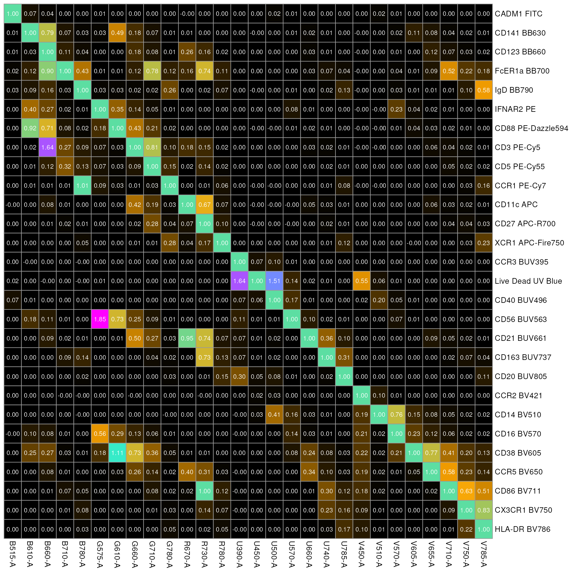
Looking at the figure, column 2: B610-A (detector for fluorophore BB630) has high spillover from flurophore: PE-Dazzle594 and PE.
In fact, when we look at the emission spectrum of the 2 dyes (PE and BB630) we see that this issue is apparent:
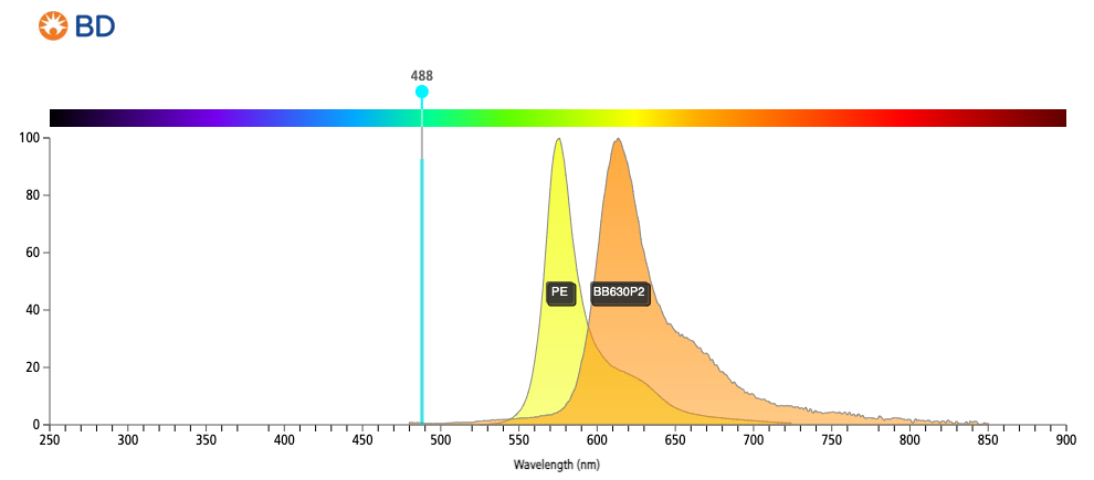 The image was created at https://www.bdbiosciences.com/en-ca/resources/bd-spectrum-viewer
using the BD spectrum viewer tool.
The image was created at https://www.bdbiosciences.com/en-ca/resources/bd-spectrum-viewer
using the BD spectrum viewer tool.
Using the spillover matrix
Now that we have a valid spillover matrix, how do we use it to correct the data?
First, we would like to highlight: SPILLOVER CORRECTION IS DONE ON THE RAW (UNTRANSFORMED) DATA.
Now to perform spillover correction (Compensation).
In the cytoverse this is done by a simple call to
compensate.
# single call to compensate
# spillover(cf)[[3]] indicates where the matrix to use lives
cf_comp <- compensate(
  x = realize_view(cf),
  spillover = spillover(cf)[[3]]
)
Transformation and visualization
Cytometry data tends to have a very high dynamic range. For example:
the range of values in PE-Cy5-5-A channel in the FCS we
have been working with is -111 2621543. The difference
between cells that do not express a marker of interest and a cell that
expresses variable level of marker could be order of magnitude. In such
a scenario, transformation of the data can aid in better
visualization and representation of the biological
phenomena.
There are multiple approaches to transform the data in
cytoverse. We will identify a few common ones as well as
demonstrate how to create new transformations.
First, let’s visualize why transformation is necessary. We go back to working with data from FR-FCM-Z5PC.
![]()
As we see, the variety of transformations aids in visualization and interpretation of the data.
Also note that the choice of transformation can and will affect the interpretation. As such, use a healthy dose of caution and follow established best practices. As well, when in doubt, talk to your collaborators.
Steps to transform data
The cytoverse libraries: flowWorkspace and
flowCore have a multiple commonly used transformations
(some are shown above) as well, one can also create a custom
transformation if required.
Let’s first use a built in transformation.
# transforming using cytoverse functions
# define a transformation
asinh_trans <- flowWorkspace::asinh_Gml2()

# create a transformList that indicates which parameters to transform
my_trans_list <- flowCore::transformList(
  from = names(
    markernames(cf)
  ),
  tfun = asinh_trans
)

# transform
cf_transformed <- flowCore::transform(
  realize_view(cf),
  my_trans_list
)![]()
Another option is to use a user defined transformation.
# define a transformation
my_trans <- function(x){
  return(sqrt(abs(x)))
}

# create a transformList
my_trans_list <- flowCore::transformList(
  from = names(
    markernames(cf)
  ),
  tfun = my_trans
)

# transform
cf_transformed <- transform(
  realize_view(cf),
  my_trans_list
)
We can also transform a set of FCS files (cytoset)
# read in a cytoset
cs <- load_cytoset_from_fcs(
  get_workshop_data(
    "fcs_data/"
  )$rpath
)

# extract per file compensation matrix into a list
compensation_list <- lapply(cytoset_to_list(cs),
                            function(x)spillover(x)[[3]])

# compensate
cs <- compensate(cs, compensation_list)

# using asinh_trans defined previously
my_trans_list <- flowCore::transformList(
  from = names(
    markernames(cf)
  ),
  tfun = asinh_trans
)

# transform: this will transform the underlying data
cs <- transform(cs,my_trans_list)
Exercise
- How can you tell if the data have been compensated? Use your
preferred plotting method to generate a scatter plot for the following
markers:
CADM1andCD141fromcfandcf_comp. You may need to transform the data for appropriate visualization. - Suppose the .fcs file does not have a spillover matrix or has an identity matrix. How confident can you be the data have been previously compensated (or not) ?
Conclusion
In this section we have described the concept of
spillover and how to use the spillover
matrix to correct for this phenomenon. As well, we described an approach
to generate the spillover matrix when it is has not be
pre-populated in the .fcs files. We also highlighted
several built-in transformations in cytoverse as well as
approaches to generate new user defined transformations. Data
transformation is topic that can require several workshops in itself. As
such, we encourage users/analyst to follow best and appropriate
practices. A highly informative reading is the following: An updated guide for
the perplexed: cytometry in the high-dimensional era.
Calculating spillover from single colour controls (optional)
You have noticed that there is no spillover matrix or an identity
matrix is present when you call spillover(cf). What can we
do to calculate the spillover matrix in this scenario?
First, verify that you have additional set of .fcs files which either have Compensation or control in the file name. These control files are generally generated as part of experiment/instrument set up before acquisition begins. If they are not available, please reach out to your collaborator or flow core manager.
Generally, there ought to be the same number of single colour controls as the number of markers being assessed + 1 unstained to estimate the background auto-fluorescence.
For demonstration purposes, we will use single colour controls from the dataset: FR-FCM-ZZ36. The data was published in this manuscript.
Here, we will make use of a csv file which maps the control files to their respective channel as well as identifies the unstained file. Note: You may need to prepare such file in advance when working with your specific experiment.
library(magrittr)

# load csv file
csv_file <- get_workshop_data(
  "control_files.csv"
)$rpath[1] %>%
read.csv(
  row.names = 1
)

# take a peek at the file
csv_file
## filename
## Alexa Fluor 405-A Compensation Controls_Alexa Fluor 405 Stained Control.fcs
## Alexa Fluor 430-A Compensation Controls_Alexa Fluor 430 Stained Control.fcs
## Alexa Fluor 488-A Compensation Controls_Alexa Fluor 488 Stained Control.fcs
## APC-A Compensation Controls_APC Stained Control.fcs
## APC-Cy7-A Compensation Controls_APC-Cy7 Stained Control.fcs
## PE-A Compensation Controls_PE Stained Control.fcs
## PE-Cy5-A Compensation Controls_PE-Cy5 Stained Control.fcs
## PE-Cy5-5-A Compensation Controls_PE-Cy5-5 Stained Control.fcs
## PE-Cy7-A Compensation Controls_PE-Cy7 Stained Control.fcs
## PE-Texas Red-A Compensation Controls_PE-Texas Red Stained Control.fcs
## PerCP-Cy5-5-A Compensation Controls_PerCP-Cy5-5 Stained Control.fcs
## Qdot 605-A Compensation Controls_Qdot 605 Stained Control.fcs
## Qdot 655-A Compensation Controls_Qdot 655 Stained Control.fcs
## Qdot 800-A Compensation Controls_Qdot 800 Stained Control.fcs
## Unstained Compensation Controls_Unstained Control.fcs
## channel
## Alexa Fluor 405-A Alexa Fluor 405-A
## Alexa Fluor 430-A Alexa Fluor 430-A
## Alexa Fluor 488-A Alexa Fluor 488-A
## APC-A APC-A
## APC-Cy7-A APC-Cy7-A
## PE-A PE-A
## PE-Cy5-A PE-Cy5-A
## PE-Cy5-5-A PE-Cy5-5-A
## PE-Cy7-A PE-Cy7-A
## PE-Texas Red-A PE-Texas Red-A
## PerCP-Cy5-5-A PerCP-Cy5-5-A
## Qdot 605-A Qdot 605-A
## Qdot 655-A Qdot 655-A
## Qdot 800-A Qdot 800-A
## Unstained Unstained
# load the set of compensation files
comp_cs <- load_cytoset_from_fcs(
  get_workshop_data(
    csv_file[["filename"]]
  )$rpath
)
sampleNames(comp_cs) <- csv_file[["channel"]]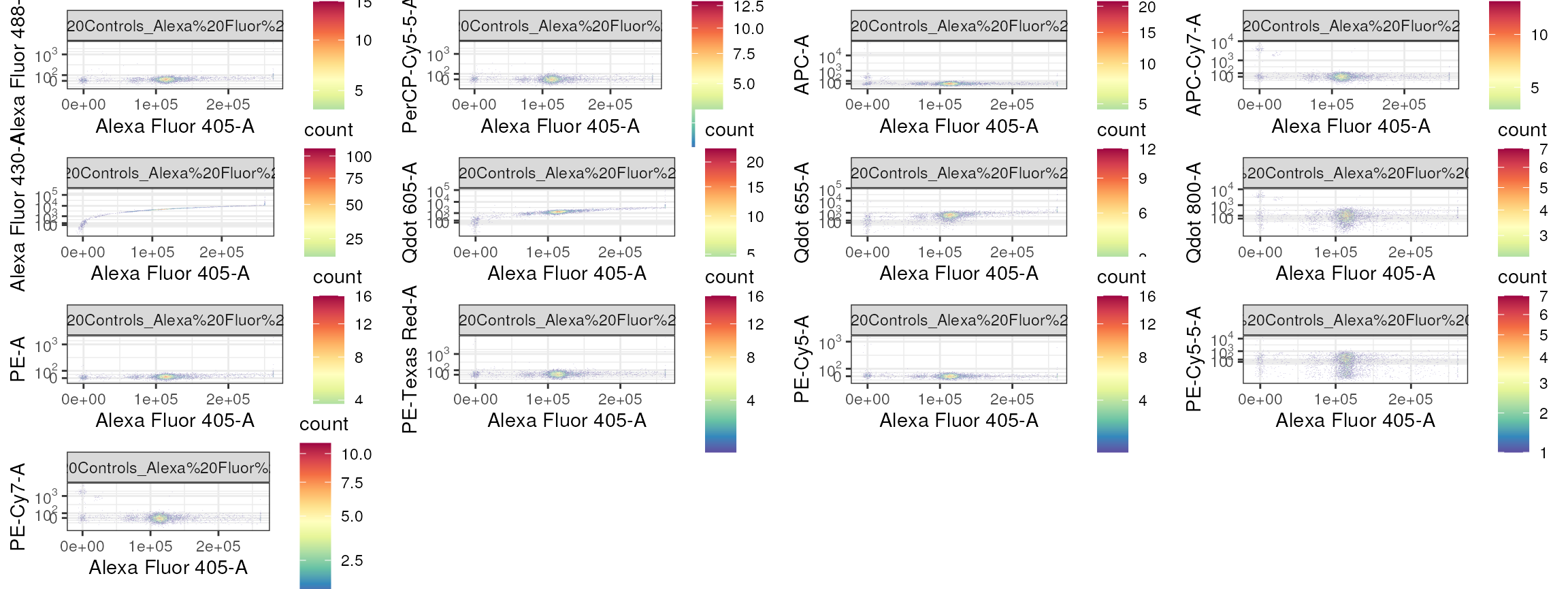
Notice that Alexa Fluor 405 is spilling heavily into Alexa Fluor 430-A and BV605-, but not into any of the other detectors.
Now, we calculate the spillover matrix using the set of controls. We
will use spillover function from flowStats
package within the cytoverse.
# calculate spillover
## using spillover from flowStats
spill <- flowStats::spillover(
  comp_cs,
  unstained = "Unstained", # indicate how the unstained file is named in flowset
  patt = "-A", # indicate which parameter should be considered
  fsc = "FSC-A",
  ssc = "SSC-A",
  stain_match = "regexpr",
  useNormFilt = TRUE
)
Now, let’s visualize the spill matrix that we calculated.
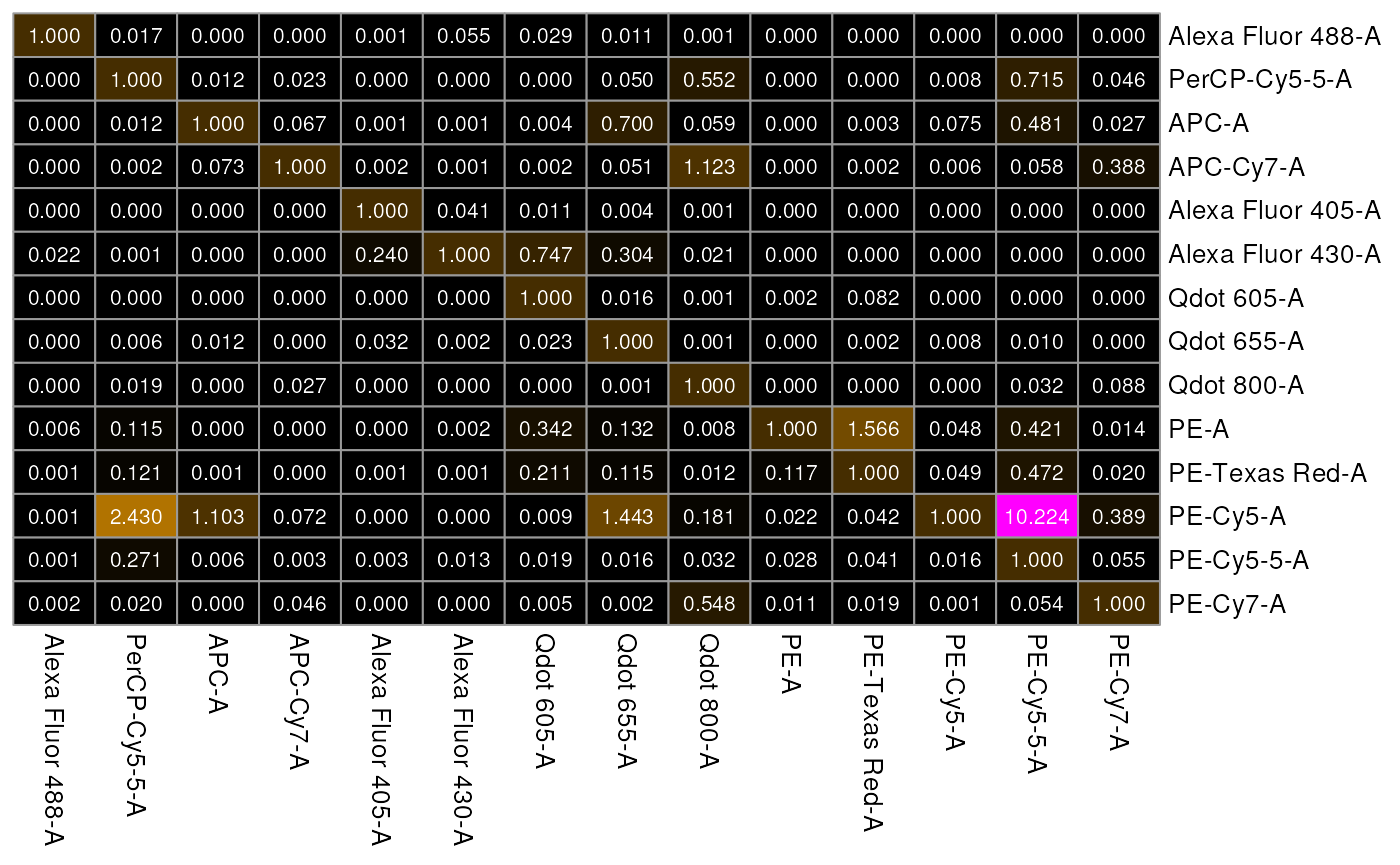
Note: Close or related fluorophores will have some degree of overlap.
Lastly, we check the effect of compensating these files.